Supported by Dr. Osamu Ogasawara and  . . |
|
Last data update: 2014.03.03 |
Data and Examples from Baltagi (2002)DescriptionThis manual page collects a list of examples from the book. Some solutions might not be exact and the list is certainly not complete. If you have suggestions for improvement (preferably in the form of code), please contact the package maintainer. ReferencesBaltagi, B.H. (2002). Econometrics, 3rd ed., Berlin: Springer-Verlag. See Also
Examples
################################
## Cigarette consumption data ##
################################
## data
data("CigarettesB", package = "AER")
## Table 3.3
cig_lm <- lm(packs ~ price, data = CigarettesB)
summary(cig_lm)
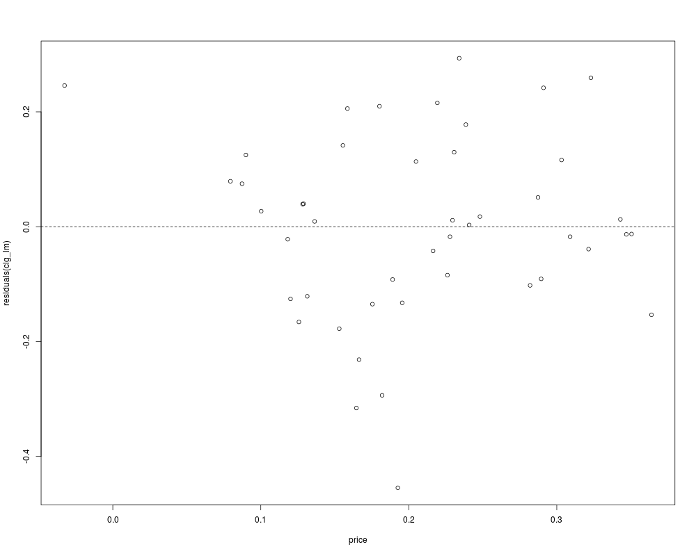
## Figure 3.9
plot(residuals(cig_lm) ~ price, data = CigarettesB)
abline(h = 0, lty = 2)
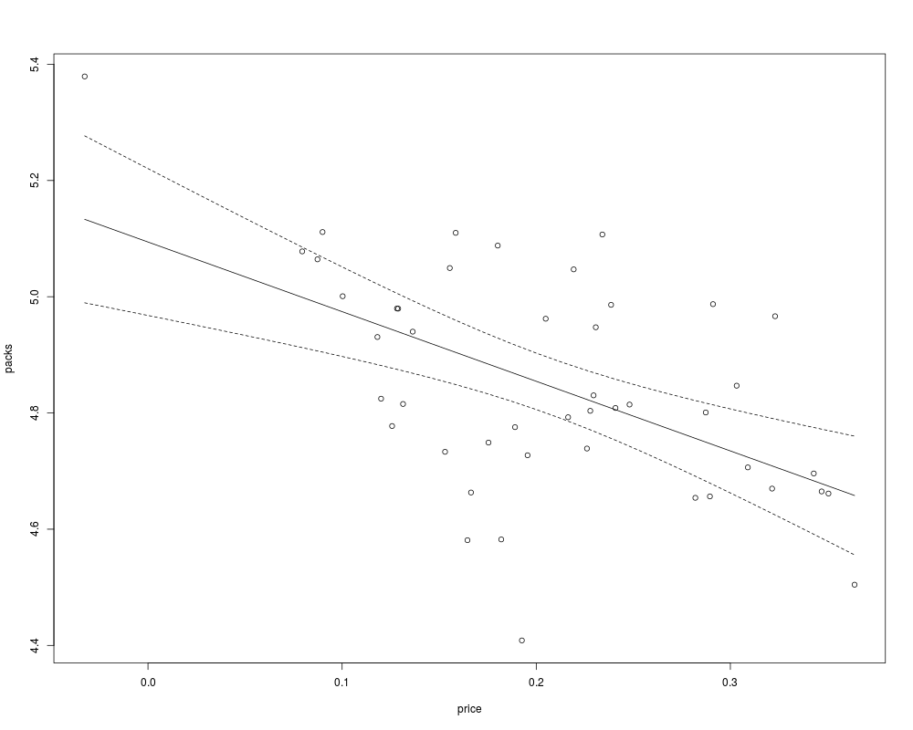
## Figure 3.10
cig_pred <- with(CigarettesB,
data.frame(price = seq(from = min(price), to = max(price), length = 30)))
cig_pred <- cbind(cig_pred, predict(cig_lm, newdata = cig_pred, interval = "confidence"))
plot(packs ~ price, data = CigarettesB)
lines(fit ~ price, data = cig_pred)
lines(lwr ~ price, data = cig_pred, lty = 2)
lines(upr ~ price, data = cig_pred, lty = 2)
## Chapter 5: diagnostic tests (p. 111-115)
cig_lm2 <- lm(packs ~ price + income, data = CigarettesB)
summary(cig_lm2)
## Glejser tests (p. 112)
ares <- abs(residuals(cig_lm2))
summary(lm(ares ~ income, data = CigarettesB))
summary(lm(ares ~ I(1/income), data = CigarettesB))
summary(lm(ares ~ I(1/sqrt(income)), data = CigarettesB))
summary(lm(ares ~ sqrt(income), data = CigarettesB))
## Goldfeld-Quandt test (p. 112)
gqtest(cig_lm2, order.by = ~ income, data = CigarettesB, fraction = 12, alternative = "less")
## NOTE: Baltagi computes the test statistic as mss1/mss2,
## i.e., tries to find decreasing variances. gqtest() always uses
## mss2/mss1 and has an "alternative" argument.
## Spearman rank correlation test (p. 113)
cor.test(~ ares + income, data = CigarettesB, method = "spearman")
## Breusch-Pagan test (p. 113)
bptest(cig_lm2, varformula = ~ income, data = CigarettesB, student = FALSE)
## White test (Table 5.1, p. 113)
bptest(cig_lm2, ~ income * price + I(income^2) + I(price^2), data = CigarettesB)
## White HC standard errors (Table 5.2, p. 114)
coeftest(cig_lm2, vcov = vcovHC(cig_lm2, type = "HC1"))
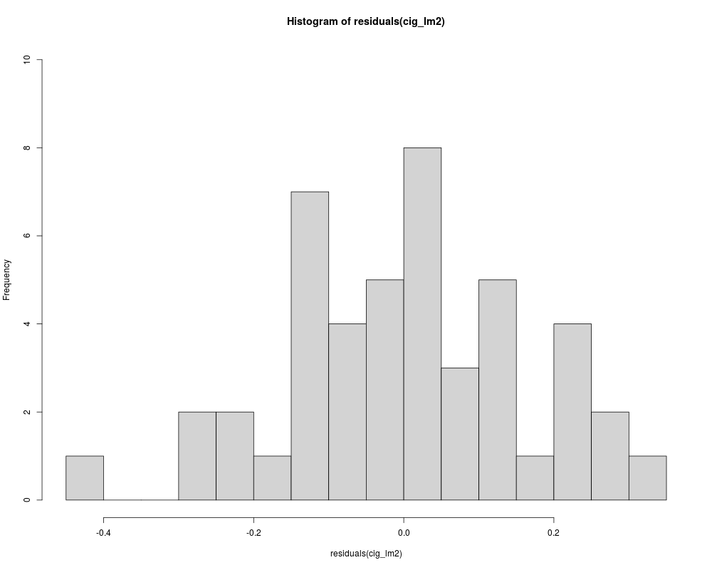
## Jarque-Bera test (Figure 5.2, p. 115)
hist(residuals(cig_lm2), breaks = 16, ylim = c(0, 10), col = "lightgray")
library("tseries")
jarque.bera.test(residuals(cig_lm2))
## Tables 8.1 and 8.2
influence.measures(cig_lm2)
#####################################
## US consumption data (1950-1993) ##
#####################################
## data
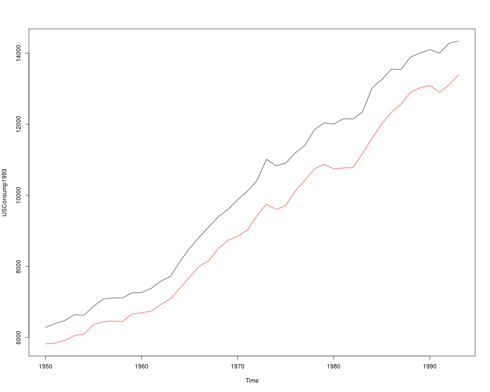
data("USConsump1993", package = "AER")
plot(USConsump1993, plot.type = "single", col = 1:2)
## Chapter 5 (p. 122-125)
fm <- lm(expenditure ~ income, data = USConsump1993)
summary(fm)
## Durbin-Watson test (p. 122)
dwtest(fm)
## Breusch-Godfrey test (Table 5.4, p. 124)
bgtest(fm)
## Newey-West standard errors (Table 5.5, p. 125)
coeftest(fm, vcov = NeweyWest(fm, lag = 3, prewhite = FALSE, adjust = TRUE))
## Chapter 8
library("strucchange")
## Recursive residuals
rr <- recresid(fm)
rr
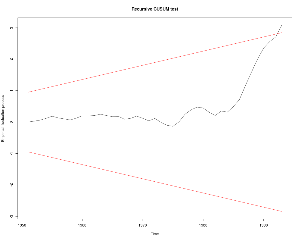
## Recursive CUSUM test
rcus <- efp(expenditure ~ income, data = USConsump1993)
plot(rcus)
sctest(rcus)
## Harvey-Collier test
harvtest(fm)
## NOTE" Mistake in Baltagi (2002) who computes
## the t-statistic incorrectly as 0.0733 via
mean(rr)/sd(rr)/sqrt(length(rr))
## whereas it should be (as in harvtest)
mean(rr)/sd(rr) * sqrt(length(rr))
## Rainbow test
raintest(fm, center = 23)
## J test for non-nested models
library("dynlm")
fm1 <- dynlm(expenditure ~ income + L(income), data = USConsump1993)
fm2 <- dynlm(expenditure ~ income + L(expenditure), data = USConsump1993)
jtest(fm1, fm2)
## Chapter 11
## Table 11.1 Instrumental-variables regression
usc <- as.data.frame(USConsump1993)
usc$investment <- usc$income - usc$expenditure
fm_ols <- lm(expenditure ~ income, data = usc)
fm_iv <- ivreg(expenditure ~ income | investment, data = usc)
## Hausman test
cf_diff <- coef(fm_iv) - coef(fm_ols)
vc_diff <- vcov(fm_iv) - vcov(fm_ols)
x2_diff <- as.vector(t(cf_diff) %*% solve(vc_diff) %*% cf_diff)
pchisq(x2_diff, df = 2, lower.tail = FALSE)
## Chapter 14
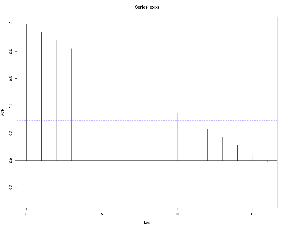
## ACF and PACF for expenditures and first differences
exps <- USConsump1993[, "expenditure"]
(acf(exps))
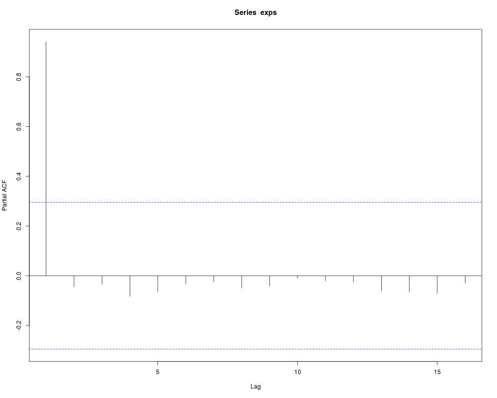
(pacf(exps))
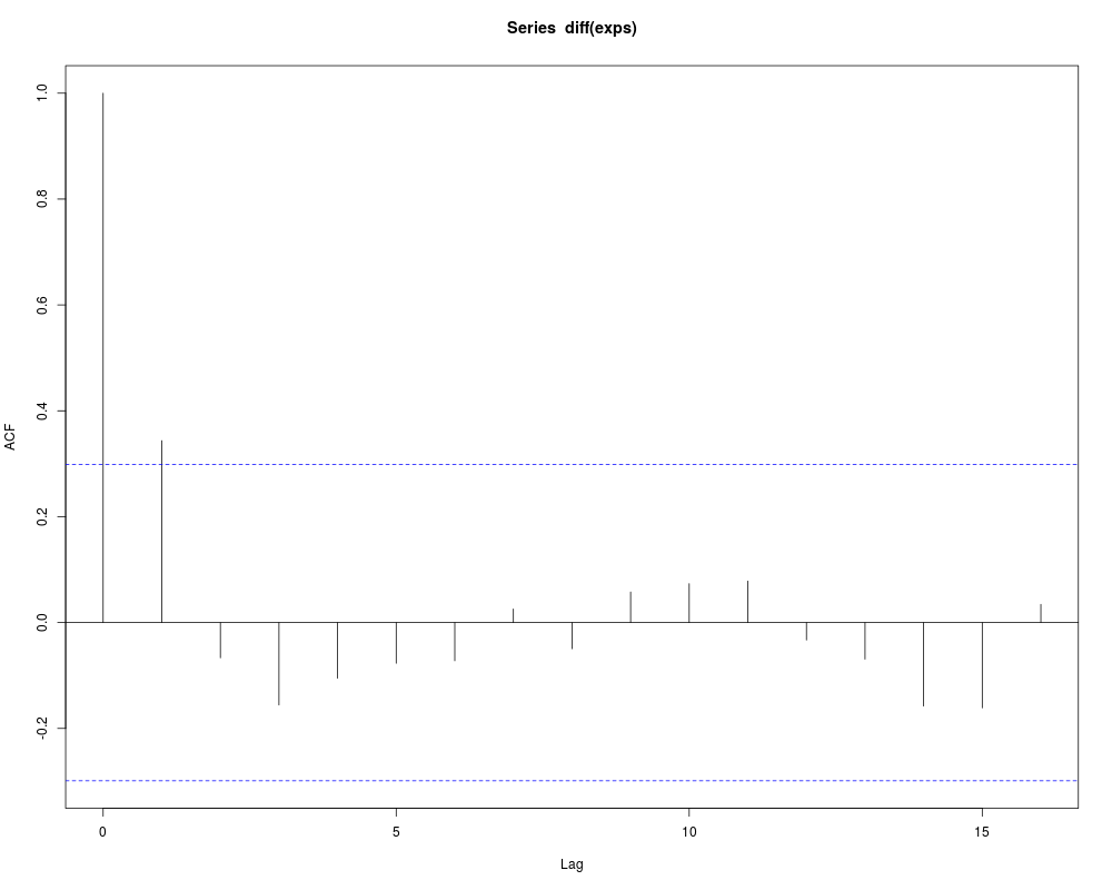
(acf(diff(exps)))
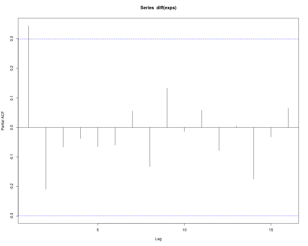
(pacf(diff(exps)))
## dynamic regressions, eq. (14.8)
fm <- dynlm(d(exps) ~ I(time(exps) - 1949) + L(exps))
summary(fm)
################################
## Grunfeld's investment data ##
################################
## select the first three companies (as panel data)
data("Grunfeld", package = "AER")
pgr <- subset(Grunfeld, firm %in% levels(Grunfeld$firm)[1:3])
library("plm")
pgr <- plm.data(pgr, c("firm", "year"))
## Ex. 10.9
library("systemfit")
gr_ols <- systemfit(invest ~ value + capital, method = "OLS", data = pgr)
gr_sur <- systemfit(invest ~ value + capital, method = "SUR", data = pgr)
#########################################
## Panel study on income dynamics 1982 ##
#########################################
## data
data("PSID1982", package = "AER")
## Table 4.1
earn_lm <- lm(log(wage) ~ . + I(experience^2), data = PSID1982)
summary(earn_lm)
## Table 13.1
union_lpm <- lm(I(as.numeric(union) - 1) ~ . - wage, data = PSID1982)
union_probit <- glm(union ~ . - wage, data = PSID1982, family = binomial(link = "probit"))
union_logit <- glm(union ~ . - wage, data = PSID1982, family = binomial)
## probit OK, logit and LPM rather different.
Results
R version 3.3.1 (2016-06-21) -- "Bug in Your Hair"
Copyright (C) 2016 The R Foundation for Statistical Computing
Platform: x86_64-pc-linux-gnu (64-bit)

R is free software and comes with ABSOLUTELY NO WARRANTY.
You are welcome to redistribute it under certain conditions.
Type 'license()' or 'licence()' for distribution details.

R is a collaborative project with many contributors.
Type 'contributors()' for more information and
'citation()' on how to cite R or R packages in publications.

Type 'demo()' for some demos, 'help()' for on-line help, or
'help.start()' for an HTML browser interface to help.
Type 'q()' to quit R.

> library(AER)
Loading required package: car
Loading required package: lmtest
Loading required package: zoo

Attaching package: 'zoo'

The following objects are masked from 'package:base':

    as.Date, as.Date.numeric

Loading required package: sandwich
Loading required package: survival
> png(filename="/home/ddbj/snapshot/RGM3/R_CC/result/AER/Baltagi2002.Rd_%03d_medium.png", width=480, height=480)
> ### Name: Baltagi2002
> ### Title: Data and Examples from Baltagi (2002)
> ### Aliases: Baltagi2002
> ### Keywords: datasets
>
> ### ** Examples
>
> ################################
> ## Cigarette consumption data ##
> ################################
>
> ## data
> data("CigarettesB", package = "AER")
>
> ## Table 3.3
> cig_lm <- lm(packs ~ price, data = CigarettesB)
> summary(cig_lm)

Call:
lm(formula = packs ~ price, data = CigarettesB)

Residuals:
     Min       1Q   Median       3Q      Max
-0.45472 -0.09968  0.00612  0.11553  0.29346

Coefficients:
            Estimate Std. Error t value Pr(>|t|)
(Intercept)   5.0941     0.0627  81.247  < 2e-16 ***
price        -1.1983     0.2818  -4.253 0.000108 ***
---
Signif. codes:  0 '***' 0.001 '**' 0.01 '*' 0.05 '.' 0.1 ' ' 1

Residual standard error: 0.163 on 44 degrees of freedom
Multiple R-squared:  0.2913,	Adjusted R-squared:  0.2752
F-statistic: 18.08 on 1 and 44 DF,  p-value: 0.0001085

>
> ## Figure 3.9
> plot(residuals(cig_lm) ~ price, data = CigarettesB)
> abline(h = 0, lty = 2)
>
> ## Figure 3.10
> cig_pred <- with(CigarettesB,
+   data.frame(price = seq(from = min(price), to = max(price), length = 30)))
> cig_pred <- cbind(cig_pred, predict(cig_lm, newdata = cig_pred, interval = "confidence"))
> plot(packs ~ price, data = CigarettesB)
> lines(fit ~ price, data = cig_pred)
> lines(lwr ~ price, data = cig_pred, lty = 2)
> lines(upr ~ price, data = cig_pred, lty = 2)
>
> ## Chapter 5: diagnostic tests (p. 111-115)
> cig_lm2 <- lm(packs ~ price + income, data = CigarettesB)
> summary(cig_lm2)

Call:
lm(formula = packs ~ price + income, data = CigarettesB)

Residuals:
     Min       1Q   Median       3Q      Max
-0.41867 -0.10683  0.00757  0.11738  0.32868

Coefficients:
            Estimate Std. Error t value Pr(>|t|)
(Intercept)   4.2997     0.9089   4.730 2.43e-05 ***
price        -1.3383     0.3246  -4.123 0.000168 ***
income        0.1724     0.1968   0.876 0.385818
---
Signif. codes:  0 '***' 0.001 '**' 0.01 '*' 0.05 '.' 0.1 ' ' 1

Residual standard error: 0.1634 on 43 degrees of freedom
Multiple R-squared:  0.3037,	Adjusted R-squared:  0.2713
F-statistic: 9.378 on 2 and 43 DF,  p-value: 0.0004168

> ## Glejser tests (p. 112)
> ares <- abs(residuals(cig_lm2))
> summary(lm(ares ~ income, data = CigarettesB))

Call:
lm(formula = ares ~ income, data = CigarettesB)

Residuals:
     Min       1Q   Median       3Q      Max
-0.13738 -0.07061 -0.01891  0.07253  0.24508

Coefficients:
            Estimate Std. Error t value Pr(>|t|)
(Intercept)  1.16169    0.46267   2.511   0.0158 *
income      -0.21689    0.09684  -2.240   0.0302 *
---
Signif. codes:  0 '***' 0.001 '**' 0.01 '*' 0.05 '.' 0.1 ' ' 1

Residual standard error: 0.09242 on 44 degrees of freedom
Multiple R-squared:  0.1023,	Adjusted R-squared:  0.08193
F-statistic: 5.016 on 1 and 44 DF,  p-value: 0.03022

> summary(lm(ares ~ I(1/income), data = CigarettesB))

Call:
lm(formula = ares ~ I(1/income), data = CigarettesB)

Residuals:
     Min       1Q   Median       3Q      Max
-0.14143 -0.07235 -0.01921  0.07227  0.24186

Coefficients:
            Estimate Std. Error t value Pr(>|t|)
(Intercept)  -0.9489     0.4671  -2.032   0.0483 *
I(1/income)   5.1287     2.2277   2.302   0.0261 *
---
Signif. codes:  0 '***' 0.001 '**' 0.01 '*' 0.05 '.' 0.1 ' ' 1

Residual standard error: 0.09215 on 44 degrees of freedom
Multiple R-squared:  0.1075,	Adjusted R-squared:  0.08722
F-statistic:   5.3 on 1 and 44 DF,  p-value: 0.02611

> summary(lm(ares ~ I(1/sqrt(income)), data = CigarettesB))

Call:
lm(formula = ares ~ I(1/sqrt(income)), data = CigarettesB)

Residuals:
     Min       1Q   Median       3Q      Max
-0.14041 -0.07192 -0.01914  0.07233  0.24267

Coefficients:
                  Estimate Std. Error t value Pr(>|t|)
(Intercept)        -2.0045     0.9317  -2.151   0.0370 *
I(1/sqrt(income))   4.6541     2.0352   2.287   0.0271 *
---
Signif. codes:  0 '***' 0.001 '**' 0.01 '*' 0.05 '.' 0.1 ' ' 1

Residual standard error: 0.09222 on 44 degrees of freedom
Multiple R-squared:  0.1062,	Adjusted R-squared:  0.08591
F-statistic: 5.229 on 1 and 44 DF,  p-value: 0.02708

> summary(lm(ares ~ sqrt(income), data = CigarettesB))

Call:
lm(formula = ares ~ sqrt(income), data = CigarettesB)

Residuals:
     Min       1Q   Median       3Q      Max
-0.13838 -0.07105 -0.01899  0.07247  0.24428

Coefficients:
             Estimate Std. Error t value Pr(>|t|)
(Intercept)    2.2172     0.9273   2.391   0.0211 *
sqrt(income)  -0.9571     0.4243  -2.255   0.0291 *
---
Signif. codes:  0 '***' 0.001 '**' 0.01 '*' 0.05 '.' 0.1 ' ' 1

Residual standard error: 0.09235 on 44 degrees of freedom
Multiple R-squared:  0.1036,	Adjusted R-squared:  0.08326
F-statistic: 5.087 on 1 and 44 DF,  p-value: 0.02913

> ## Goldfeld-Quandt test (p. 112)
> gqtest(cig_lm2, order.by = ~ income, data = CigarettesB, fraction = 12, alternative = "less")

	Goldfeld-Quandt test

data:  cig_lm2
GQ = 0.31846, df1 = 14, df2 = 14, p-value = 0.02017

> ## NOTE: Baltagi computes the test statistic as mss1/mss2,
> ## i.e., tries to find decreasing variances. gqtest() always uses
> ## mss2/mss1 and has an "alternative" argument.
>
> ## Spearman rank correlation test (p. 113)
> cor.test(~ ares + income, data = CigarettesB, method = "spearman")

	Spearman's rank correlation rho

data:  ares and income
S = 20784, p-value = 0.05813
alternative hypothesis: true rho is not equal to 0
sample estimates:
       rho
-0.2817761

> ## Breusch-Pagan test (p. 113)
> bptest(cig_lm2, varformula = ~ income, data = CigarettesB, student = FALSE)

	Breusch-Pagan test

data:  cig_lm2
BP = 5.4852, df = 1, p-value = 0.01918

> ## White test (Table 5.1, p. 113)
> bptest(cig_lm2, ~ income * price + I(income^2) + I(price^2), data = CigarettesB)

	studentized Breusch-Pagan test

data:  cig_lm2
BP = 15.656, df = 5, p-value = 0.007897

> ## White HC standard errors (Table 5.2, p. 114)
> coeftest(cig_lm2, vcov = vcovHC(cig_lm2, type = "HC1"))

t test of coefficients:

            Estimate Std. Error t value  Pr(>|t|)
(Intercept)  4.29966    1.09523  3.9258 0.0003076 ***
price       -1.33833    0.34337 -3.8977 0.0003352 ***
income       0.17239    0.23661  0.7286 0.4702172
---
Signif. codes:  0 '***' 0.001 '**' 0.01 '*' 0.05 '.' 0.1 ' ' 1

> ## Jarque-Bera test (Figure 5.2, p. 115)
> hist(residuals(cig_lm2), breaks = 16, ylim = c(0, 10), col = "lightgray")
> library("tseries")
> jarque.bera.test(residuals(cig_lm2))

	Jarque Bera Test

data:  residuals(cig_lm2)
X-squared = 0.28935, df = 2, p-value = 0.8653

>
> ## Tables 8.1 and 8.2
> influence.measures(cig_lm2)
Influence measures of
	 lm(formula = packs ~ price + income, data = CigarettesB) :

     dfb.1_  dfb.pric dfb.incm    dffit cov.r   cook.d    hat inf
AL  0.14503  0.069010 -0.14188  0.19186 1.070 1.23e-02 0.0480
AZ -0.11311  0.033072  0.10173 -0.25077 0.968 2.05e-02 0.0315
AR  0.56419  0.376064 -0.56381  0.66702 0.847 1.36e-01 0.0847
CA -0.01386 -0.255192  0.02769 -0.31637 1.114 3.34e-02 0.0975
CT  0.15244 -0.022453 -0.14793 -0.20087 1.219 1.37e-02 0.1354   *
DE -0.12654 -0.037389  0.12991  0.23129 0.992 1.76e-02 0.0326
DC  0.23239  0.001472 -0.22823 -0.29167 1.149 2.86e-02 0.1104
FL  0.01116  0.050233 -0.01301  0.07389 1.112 1.86e-03 0.0431
GA -0.00269 -0.028971  0.00551  0.04527 1.114 6.99e-04 0.0402
ID -0.10101 -0.013791  0.09591 -0.15005 1.079 7.59e-03 0.0413
IL -0.00101  0.000075  0.00101  0.00178 1.118 1.09e-06 0.0399
IN -0.03076 -0.153574  0.04353  0.19363 1.105 1.26e-02 0.0650
IA  0.00638  0.007696 -0.00639  0.01509 1.107 7.77e-05 0.0310
KS  0.00314 -0.002575 -0.00389 -0.04083 1.092 5.68e-04 0.0223
KY -0.09222 -0.725107  0.14758  0.80979 1.113 2.10e-01 0.1977   *
LA  0.31705  0.226157 -0.31744  0.38745 1.022 4.91e-02 0.0761
ME  0.17424  0.309538 -0.18410  0.40000 0.940 5.13e-02 0.0553
MD  0.39398  0.378023 -0.41346 -0.50701 1.073 8.40e-02 0.1216
MA  0.19840  0.073723 -0.20018 -0.23411 1.126 1.84e-02 0.0856
MI -0.00898  0.025355  0.00991  0.12316 1.052 5.10e-03 0.0238
MN  0.01342  0.042769 -0.01537  0.05001 1.172 8.53e-04 0.0864
MS  0.06675  0.002382 -0.06369  0.08277 1.171 2.33e-03 0.0883
MO -0.03986 -0.089643  0.04634  0.10541 1.154 3.78e-03 0.0787
MT -0.04820  0.067706  0.03769 -0.19283 1.021 1.24e-02 0.0312
NE  0.02185  0.027580 -0.02540 -0.09498 1.072 3.05e-03 0.0243
NV  0.05366  0.347879 -0.06990  0.45042 0.937 6.47e-02 0.0646
NH -0.34967 -0.257318  0.36079  0.40764 1.142 5.53e-02 0.1308
NJ  0.12527 -0.004859 -0.12241 -0.15616 1.234 8.29e-03 0.1394   *
NM -0.38923 -0.064661  0.37379 -0.49010 0.901 7.56e-02 0.0639
NY  0.01626 -0.028925 -0.01431 -0.05033 1.175 8.64e-04 0.0888
ND -0.15387 -0.005358  0.14232 -0.31360 0.885 3.12e-02 0.0295
OH -0.00856 -0.028773  0.01108  0.04159 1.117 5.90e-04 0.0423
OK -0.12028 -0.047228  0.11708 -0.15599 1.094 8.21e-03 0.0505
PA  0.00741 -0.001370 -0.00765 -0.02452 1.100 2.05e-04 0.0257
RI  0.00218  0.114469 -0.00738  0.16917 1.088 9.64e-03 0.0504
SC  0.04282 -0.092254 -0.03271  0.15382 1.132 8.02e-03 0.0725
SD -0.04178  0.064802  0.03307 -0.14581 1.079 7.17e-03 0.0402
TN  0.01884 -0.062711 -0.01037  0.15431 1.046 7.98e-03 0.0294
TX -0.06472 -0.095510  0.06734 -0.12671 1.113 5.44e-03 0.0546
UT -0.77803 -0.317059  0.76368 -0.88760 0.679 2.24e-01 0.0856   *
VT -0.02396 -0.065794  0.03278  0.20305 0.979 1.35e-02 0.0243
VA  0.05235  0.069110 -0.05673 -0.08713 1.156 2.59e-03 0.0773
WA -0.00136 -0.010137  0.00187 -0.01242 1.175 5.27e-05 0.0866
WV -0.11903  0.031391  0.11039 -0.17766 1.122 1.07e-02 0.0709
WI  0.00494  0.006306 -0.00481  0.01736 1.100 1.03e-04 0.0254
WY -0.00156 -0.025435  0.00388  0.03501 1.135 4.18e-04 0.0555
>
>
> #####################################
> ## US consumption data (1950-1993) ##
> #####################################
>
> ## data
> data("USConsump1993", package = "AER")
> plot(USConsump1993, plot.type = "single", col = 1:2)
>
> ## Chapter 5 (p. 122-125)
> fm <- lm(expenditure ~ income, data = USConsump1993)
> summary(fm)

Call:
lm(formula = expenditure ~ income, data = USConsump1993)

Residuals:
    Min      1Q  Median      3Q     Max
-294.52  -67.02    4.64   90.02  325.84

Coefficients:
              Estimate Std. Error t value Pr(>|t|)
(Intercept) -65.795821  90.990824  -0.723    0.474
income        0.915623   0.008648 105.874   <2e-16 ***
---
Signif. codes:  0 '***' 0.001 '**' 0.01 '*' 0.05 '.' 0.1 ' ' 1

Residual standard error: 153.6 on 42 degrees of freedom
Multiple R-squared:  0.9963,	Adjusted R-squared:  0.9962
F-statistic: 1.121e+04 on 1 and 42 DF,  p-value: < 2.2e-16

> ## Durbin-Watson test (p. 122)
> dwtest(fm)

	Durbin-Watson test

data:  fm
DW = 0.46078, p-value = 3.274e-11
alternative hypothesis: true autocorrelation is greater than 0

> ## Breusch-Godfrey test (Table 5.4, p. 124)
> bgtest(fm)

	Breusch-Godfrey test for serial correlation of order up to 1

data:  fm
LM test = 24.901, df = 1, p-value = 6.034e-07

> ## Newey-West standard errors (Table 5.5, p. 125)
> coeftest(fm, vcov = NeweyWest(fm, lag = 3, prewhite = FALSE, adjust = TRUE))

t test of coefficients:

              Estimate Std. Error t value Pr(>|t|)
(Intercept) -65.795821 133.345400 -0.4934   0.6243
income        0.915623   0.015458 59.2319   <2e-16 ***
---
Signif. codes:  0 '***' 0.001 '**' 0.01 '*' 0.05 '.' 0.1 ' ' 1

>
> ## Chapter 8
> library("strucchange")
> ## Recursive residuals
> rr <- recresid(fm)
> rr
 [1]   24.900681   30.354827   50.893291   63.260389  -49.805907  -28.404311
 [7]  -31.520559   53.194256   67.696114   -2.646556    9.679147   39.658827
[13]  -40.126557  -30.260756    2.605633  -78.941467   27.185066   64.363195
[19]  -64.906717  -71.641013   70.095867 -113.475323  -85.633171  -29.427630
[25]  128.328459  220.693133  126.591749   78.394247  -25.955574 -124.178686
[31]  -90.845193  127.830581  -30.794629  159.780872  201.707127  405.310561
[37]  390.953841  373.370919  316.431235  188.109683  134.461285  339.300414
> ## Recursive CUSUM test
> rcus <- efp(expenditure ~ income, data = USConsump1993)
> plot(rcus)
> sctest(rcus)

	Recursive CUSUM test

data:  rcus
S = 1.0267, p-value = 0.02707

> ## Harvey-Collier test
> harvtest(fm)

	Harvey-Collier test

data:  fm
HC = 3.0802, df = 41, p-value = 0.003685

> ## NOTE" Mistake in Baltagi (2002) who computes
> ## the t-statistic incorrectly as 0.0733 via
> mean(rr)/sd(rr)/sqrt(length(rr))
[1] 0.07333754
> ## whereas it should be (as in harvtest)
> mean(rr)/sd(rr) * sqrt(length(rr))
[1] 3.080177
>
> ## Rainbow test
> raintest(fm, center = 23)

	Rainbow test

data:  fm
Rain = 4.1448, df1 = 22, df2 = 20, p-value = 0.001116

>
> ## J test for non-nested models
> library("dynlm")
> fm1 <- dynlm(expenditure ~ income + L(income), data = USConsump1993)
> fm2 <- dynlm(expenditure ~ income + L(expenditure), data = USConsump1993)
> jtest(fm1, fm2)
J test

Model 1: expenditure ~ income + L(income)
Model 2: expenditure ~ income + L(expenditure)
                Estimate Std. Error t value  Pr(>|t|)
M1 + fitted(M2)   1.6378    0.20984  7.8051 1.726e-09 ***
M2 + fitted(M1)  -2.5419    0.61603 -4.1262 0.0001874 ***
---
Signif. codes:  0 '***' 0.001 '**' 0.01 '*' 0.05 '.' 0.1 ' ' 1
>
> ## Chapter 11
> ## Table 11.1 Instrumental-variables regression
> usc <- as.data.frame(USConsump1993)
> usc$investment <- usc$income - usc$expenditure
> fm_ols <- lm(expenditure ~ income, data = usc)
> fm_iv <- ivreg(expenditure ~ income | investment, data = usc)
> ## Hausman test
> cf_diff <- coef(fm_iv) - coef(fm_ols)
> vc_diff <- vcov(fm_iv) - vcov(fm_ols)
> x2_diff <- as.vector(t(cf_diff) %*% solve(vc_diff) %*% cf_diff)
> pchisq(x2_diff, df = 2, lower.tail = FALSE)
[1] 0.0001836953
>
> ## Chapter 14
> ## ACF and PACF for expenditures and first differences
> exps <- USConsump1993[, "expenditure"]
> (acf(exps))

Autocorrelations of series 'exps', by lag

     0      1      2      3      4      5      6      7      8      9     10
 1.000  0.941  0.880  0.820  0.753  0.683  0.614  0.547  0.479  0.412  0.348
    11     12     13     14     15     16
 0.288  0.230  0.171  0.110  0.049 -0.010
> (pacf(exps))

Partial autocorrelations of series 'exps', by lag

     1      2      3      4      5      6      7      8      9     10     11
 0.941 -0.045 -0.035 -0.083 -0.064 -0.034 -0.025 -0.049 -0.043 -0.011 -0.022
    12     13     14     15     16
-0.025 -0.061 -0.066 -0.071 -0.030
> (acf(diff(exps)))

Autocorrelations of series 'diff(exps)', by lag

     0      1      2      3      4      5      6      7      8      9     10
 1.000  0.344 -0.067 -0.156 -0.105 -0.077 -0.072  0.026 -0.050  0.058  0.073
    11     12     13     14     15     16
 0.078 -0.033 -0.069 -0.158 -0.161  0.034
> (pacf(diff(exps)))

Partial autocorrelations of series 'diff(exps)', by lag

     1      2      3      4      5      6      7      8      9     10     11
 0.344 -0.209 -0.066 -0.038 -0.065 -0.060  0.056 -0.133  0.133 -0.014  0.058
    12     13     14     15     16
-0.079  0.005 -0.175 -0.032  0.065
>
> ## dynamic regressions, eq. (14.8)
> fm <- dynlm(d(exps) ~ I(time(exps) - 1949) + L(exps))
> summary(fm)

Time series regression with "ts" data:
Start = 1951, End = 1993

Call:
dynlm(formula = d(exps) ~ I(time(exps) - 1949) + L(exps))

Residuals:
    Min      1Q  Median      3Q     Max
-357.76  -78.18   22.49  108.97  201.06

Coefficients:
                       Estimate Std. Error t value Pr(>|t|)
(Intercept)          1048.96039  353.81291   2.965  0.00509 **
I(time(exps) - 1949)   39.90164   14.31344   2.788  0.00808 **
L(exps)                -0.19561    0.07398  -2.644  0.01164 *
---
Signif. codes:  0 '***' 0.001 '**' 0.01 '*' 0.05 '.' 0.1 ' ' 1

Residual standard error: 147.4 on 40 degrees of freedom
Multiple R-squared:  0.1784,	Adjusted R-squared:  0.1373
F-statistic: 4.343 on 2 and 40 DF,  p-value: 0.01963

>
>
> ################################
> ## Grunfeld's investment data ##
> ################################
>
> ## select the first three companies (as panel data)
> data("Grunfeld", package = "AER")
> pgr <- subset(Grunfeld, firm %in% levels(Grunfeld$firm)[1:3])
> library("plm")
Loading required package: Formula
> pgr <- plm.data(pgr, c("firm", "year"))
>
> ## Ex. 10.9
> library("systemfit")
Loading required package: Matrix
> gr_ols <- systemfit(invest ~ value + capital, method = "OLS", data = pgr)
> gr_sur <- systemfit(invest ~ value + capital, method = "SUR", data = pgr)
>
>
> #########################################
> ## Panel study on income dynamics 1982 ##
> #########################################
>
> ## data
> data("PSID1982", package = "AER")
>
> ## Table 4.1
> earn_lm <- lm(log(wage) ~ . + I(experience^2), data = PSID1982)
> summary(earn_lm)

Call:
lm(formula = log(wage) ~ . + I(experience^2), data = PSID1982)

Residuals:
    Min      1Q  Median      3Q     Max
-1.0271 -0.2292  0.0155  0.2231  1.1314

Coefficients:
                  Estimate Std. Error t value Pr(>|t|)
(Intercept)      5.5900930  0.1901125  29.404  < 2e-16 ***
experience       0.0293801  0.0065241   4.503 8.09e-06 ***
weeks            0.0034128  0.0026776   1.275 0.202973
occupationblue  -0.1615216  0.0369073  -4.376 1.43e-05 ***
industryyes      0.0846626  0.0291637   2.903 0.003836 **
southyes        -0.0587635  0.0309069  -1.901 0.057755 .
smsayes          0.1661912  0.0295510   5.624 2.90e-08 ***
marriedyes       0.0952370  0.0489277   1.946 0.052077 .
genderfemale    -0.3245574  0.0607294  -5.344 1.30e-07 ***
unionyes         0.1062775  0.0316755   3.355 0.000845 ***
education        0.0571935  0.0065910   8.678  < 2e-16 ***
ethnicityafam   -0.1904220  0.0544118  -3.500 0.000502 ***
I(experience^2) -0.0004860  0.0001268  -3.833 0.000141 ***
---
Signif. codes:  0 '***' 0.001 '**' 0.01 '*' 0.05 '.' 0.1 ' ' 1

Residual standard error: 0.3256 on 582 degrees of freedom
Multiple R-squared:  0.4597,	Adjusted R-squared:  0.4485
F-statistic: 41.26 on 12 and 582 DF,  p-value: < 2.2e-16

>
> ## Table 13.1
> union_lpm <- lm(I(as.numeric(union) - 1) ~ . - wage, data = PSID1982)
> union_probit <- glm(union ~ . - wage, data = PSID1982, family = binomial(link = "probit"))
> union_logit <- glm(union ~ . - wage, data = PSID1982, family = binomial)
> ## probit OK, logit and LPM rather different.
>
>
>
>
>
> dev.off()
null device
          1
>
|
Created & Maintained by Osamu Ogasawara (osamu.ogasawara@gmail.com) and 