Supported by Dr. Osamu Ogasawara and  . . |
|
Last data update: 2014.03.03 |
Cigarette Consumption DataDescriptionCross-section data on cigarette consumption for 46 US States, for the year 1992. Usagedata("CigarettesB")
FormatA data frame containing 46 observations on 3 variables.
SourceThe data are from Baltagi (2002). ReferencesBaltagi, B.H. (2002). Econometrics, 3rd ed. Berlin, Springer. Baltagi, B.H. and Levin, D. (1992). Cigarette Taxation: Raising Revenues and Reducing Consumption. Structural Change and Economic Dynamics, 3, 321–335. See Also
Examples
data("CigarettesB")
## Baltagi (2002)
## Table 3.3
cig_lm <- lm(packs ~ price, data = CigarettesB)
summary(cig_lm)
## Chapter 5: diagnostic tests (p. 111-115)
cig_lm2 <- lm(packs ~ price + income, data = CigarettesB)
summary(cig_lm2)
## Glejser tests (p. 112)
ares <- abs(residuals(cig_lm2))
summary(lm(ares ~ income, data = CigarettesB))
summary(lm(ares ~ I(1/income), data = CigarettesB))
summary(lm(ares ~ I(1/sqrt(income)), data = CigarettesB))
summary(lm(ares ~ sqrt(income), data = CigarettesB))
## Goldfeld-Quandt test (p. 112)
gqtest(cig_lm2, order.by = ~ income, data = CigarettesB, fraction = 12, alternative = "less")
## NOTE: Baltagi computes the test statistic as mss1/mss2,
## i.e., tries to find decreasing variances. gqtest() always uses
## mss2/mss1 and has an "alternative" argument.
## Spearman rank correlation test (p. 113)
cor.test(~ ares + income, data = CigarettesB, method = "spearman")
## Breusch-Pagan test (p. 113)
bptest(cig_lm2, varformula = ~ income, data = CigarettesB, student = FALSE)
## White test (Table 5.1, p. 113)
bptest(cig_lm2, ~ income * price + I(income^2) + I(price^2), data = CigarettesB)
## White HC standard errors (Table 5.2, p. 114)
coeftest(cig_lm2, vcov = vcovHC(cig_lm2, type = "HC1"))
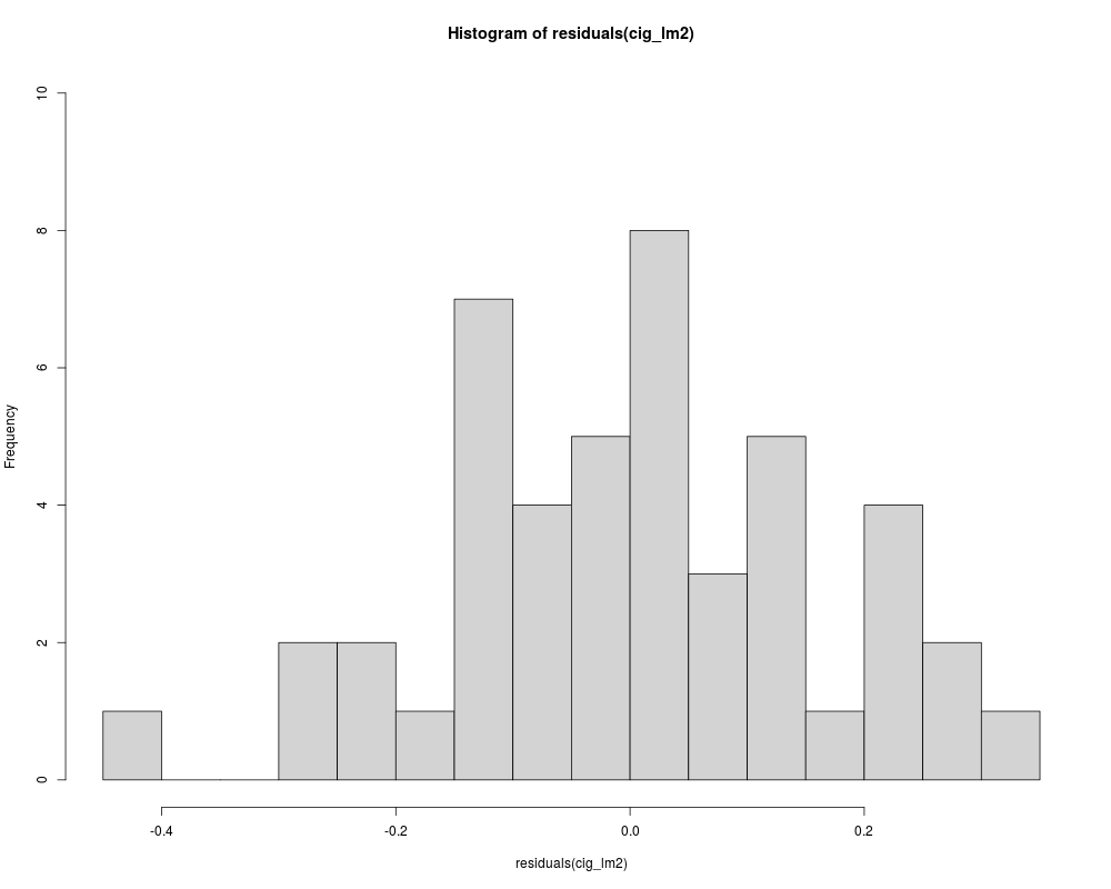
## Jarque-Bera test (Figure 5.2, p. 115)
hist(residuals(cig_lm2), breaks = 16, ylim = c(0, 10), col = "lightgray")
library("tseries")
jarque.bera.test(residuals(cig_lm2))
## Tables 8.1 and 8.2
influence.measures(cig_lm2)
## More examples can be found in:
## help("Baltagi2002")
Results
R version 3.3.1 (2016-06-21) -- "Bug in Your Hair"
Copyright (C) 2016 The R Foundation for Statistical Computing
Platform: x86_64-pc-linux-gnu (64-bit)

R is free software and comes with ABSOLUTELY NO WARRANTY.
You are welcome to redistribute it under certain conditions.
Type 'license()' or 'licence()' for distribution details.

R is a collaborative project with many contributors.
Type 'contributors()' for more information and
'citation()' on how to cite R or R packages in publications.

Type 'demo()' for some demos, 'help()' for on-line help, or
'help.start()' for an HTML browser interface to help.
Type 'q()' to quit R.

> library(AER)
Loading required package: car
Loading required package: lmtest
Loading required package: zoo

Attaching package: 'zoo'

The following objects are masked from 'package:base':

    as.Date, as.Date.numeric

Loading required package: sandwich
Loading required package: survival
> png(filename="/home/ddbj/snapshot/RGM3/R_CC/result/AER/CigarettesB.Rd_%03d_medium.png", width=480, height=480)
> ### Name: CigarettesB
> ### Title: Cigarette Consumption Data
> ### Aliases: CigarettesB
> ### Keywords: datasets
>
> ### ** Examples
>
> data("CigarettesB")
>
> ## Baltagi (2002)
> ## Table 3.3
> cig_lm <- lm(packs ~ price, data = CigarettesB)
> summary(cig_lm)

Call:
lm(formula = packs ~ price, data = CigarettesB)

Residuals:
     Min       1Q   Median       3Q      Max
-0.45472 -0.09968  0.00612  0.11553  0.29346

Coefficients:
            Estimate Std. Error t value Pr(>|t|)
(Intercept)   5.0941     0.0627  81.247  < 2e-16 ***
price        -1.1983     0.2818  -4.253 0.000108 ***
---
Signif. codes:  0 '***' 0.001 '**' 0.01 '*' 0.05 '.' 0.1 ' ' 1

Residual standard error: 0.163 on 44 degrees of freedom
Multiple R-squared:  0.2913,	Adjusted R-squared:  0.2752
F-statistic: 18.08 on 1 and 44 DF,  p-value: 0.0001085

>
> ## Chapter 5: diagnostic tests (p. 111-115)
> cig_lm2 <- lm(packs ~ price + income, data = CigarettesB)
> summary(cig_lm2)

Call:
lm(formula = packs ~ price + income, data = CigarettesB)

Residuals:
     Min       1Q   Median       3Q      Max
-0.41867 -0.10683  0.00757  0.11738  0.32868

Coefficients:
            Estimate Std. Error t value Pr(>|t|)
(Intercept)   4.2997     0.9089   4.730 2.43e-05 ***
price        -1.3383     0.3246  -4.123 0.000168 ***
income        0.1724     0.1968   0.876 0.385818
---
Signif. codes:  0 '***' 0.001 '**' 0.01 '*' 0.05 '.' 0.1 ' ' 1

Residual standard error: 0.1634 on 43 degrees of freedom
Multiple R-squared:  0.3037,	Adjusted R-squared:  0.2713
F-statistic: 9.378 on 2 and 43 DF,  p-value: 0.0004168

> ## Glejser tests (p. 112)
> ares <- abs(residuals(cig_lm2))
> summary(lm(ares ~ income, data = CigarettesB))

Call:
lm(formula = ares ~ income, data = CigarettesB)

Residuals:
     Min       1Q   Median       3Q      Max
-0.13738 -0.07061 -0.01891  0.07253  0.24508

Coefficients:
            Estimate Std. Error t value Pr(>|t|)
(Intercept)  1.16169    0.46267   2.511   0.0158 *
income      -0.21689    0.09684  -2.240   0.0302 *
---
Signif. codes:  0 '***' 0.001 '**' 0.01 '*' 0.05 '.' 0.1 ' ' 1

Residual standard error: 0.09242 on 44 degrees of freedom
Multiple R-squared:  0.1023,	Adjusted R-squared:  0.08193
F-statistic: 5.016 on 1 and 44 DF,  p-value: 0.03022

> summary(lm(ares ~ I(1/income), data = CigarettesB))

Call:
lm(formula = ares ~ I(1/income), data = CigarettesB)

Residuals:
     Min       1Q   Median       3Q      Max
-0.14143 -0.07235 -0.01921  0.07227  0.24186

Coefficients:
            Estimate Std. Error t value Pr(>|t|)
(Intercept)  -0.9489     0.4671  -2.032   0.0483 *
I(1/income)   5.1287     2.2277   2.302   0.0261 *
---
Signif. codes:  0 '***' 0.001 '**' 0.01 '*' 0.05 '.' 0.1 ' ' 1

Residual standard error: 0.09215 on 44 degrees of freedom
Multiple R-squared:  0.1075,	Adjusted R-squared:  0.08722
F-statistic:   5.3 on 1 and 44 DF,  p-value: 0.02611

> summary(lm(ares ~ I(1/sqrt(income)), data = CigarettesB))

Call:
lm(formula = ares ~ I(1/sqrt(income)), data = CigarettesB)

Residuals:
     Min       1Q   Median       3Q      Max
-0.14041 -0.07192 -0.01914  0.07233  0.24267

Coefficients:
                  Estimate Std. Error t value Pr(>|t|)
(Intercept)        -2.0045     0.9317  -2.151   0.0370 *
I(1/sqrt(income))   4.6541     2.0352   2.287   0.0271 *
---
Signif. codes:  0 '***' 0.001 '**' 0.01 '*' 0.05 '.' 0.1 ' ' 1

Residual standard error: 0.09222 on 44 degrees of freedom
Multiple R-squared:  0.1062,	Adjusted R-squared:  0.08591
F-statistic: 5.229 on 1 and 44 DF,  p-value: 0.02708

> summary(lm(ares ~ sqrt(income), data = CigarettesB))

Call:
lm(formula = ares ~ sqrt(income), data = CigarettesB)

Residuals:
     Min       1Q   Median       3Q      Max
-0.13838 -0.07105 -0.01899  0.07247  0.24428

Coefficients:
             Estimate Std. Error t value Pr(>|t|)
(Intercept)    2.2172     0.9273   2.391   0.0211 *
sqrt(income)  -0.9571     0.4243  -2.255   0.0291 *
---
Signif. codes:  0 '***' 0.001 '**' 0.01 '*' 0.05 '.' 0.1 ' ' 1

Residual standard error: 0.09235 on 44 degrees of freedom
Multiple R-squared:  0.1036,	Adjusted R-squared:  0.08326
F-statistic: 5.087 on 1 and 44 DF,  p-value: 0.02913

> ## Goldfeld-Quandt test (p. 112)
> gqtest(cig_lm2, order.by = ~ income, data = CigarettesB, fraction = 12, alternative = "less")

	Goldfeld-Quandt test

data:  cig_lm2
GQ = 0.31846, df1 = 14, df2 = 14, p-value = 0.02017

> ## NOTE: Baltagi computes the test statistic as mss1/mss2,
> ## i.e., tries to find decreasing variances. gqtest() always uses
> ## mss2/mss1 and has an "alternative" argument.
>
> ## Spearman rank correlation test (p. 113)
> cor.test(~ ares + income, data = CigarettesB, method = "spearman")

	Spearman's rank correlation rho

data:  ares and income
S = 20784, p-value = 0.05813
alternative hypothesis: true rho is not equal to 0
sample estimates:
       rho
-0.2817761

> ## Breusch-Pagan test (p. 113)
> bptest(cig_lm2, varformula = ~ income, data = CigarettesB, student = FALSE)

	Breusch-Pagan test

data:  cig_lm2
BP = 5.4852, df = 1, p-value = 0.01918

> ## White test (Table 5.1, p. 113)
> bptest(cig_lm2, ~ income * price + I(income^2) + I(price^2), data = CigarettesB)

	studentized Breusch-Pagan test

data:  cig_lm2
BP = 15.656, df = 5, p-value = 0.007897

> ## White HC standard errors (Table 5.2, p. 114)
> coeftest(cig_lm2, vcov = vcovHC(cig_lm2, type = "HC1"))

t test of coefficients:

            Estimate Std. Error t value  Pr(>|t|)
(Intercept)  4.29966    1.09523  3.9258 0.0003076 ***
price       -1.33833    0.34337 -3.8977 0.0003352 ***
income       0.17239    0.23661  0.7286 0.4702172
---
Signif. codes:  0 '***' 0.001 '**' 0.01 '*' 0.05 '.' 0.1 ' ' 1

> ## Jarque-Bera test (Figure 5.2, p. 115)
> hist(residuals(cig_lm2), breaks = 16, ylim = c(0, 10), col = "lightgray")
> library("tseries")
> jarque.bera.test(residuals(cig_lm2))

	Jarque Bera Test

data:  residuals(cig_lm2)
X-squared = 0.28935, df = 2, p-value = 0.8653

>
> ## Tables 8.1 and 8.2
> influence.measures(cig_lm2)
Influence measures of
	 lm(formula = packs ~ price + income, data = CigarettesB) :

     dfb.1_  dfb.pric dfb.incm    dffit cov.r   cook.d    hat inf
AL  0.14503  0.069010 -0.14188  0.19186 1.070 1.23e-02 0.0480
AZ -0.11311  0.033072  0.10173 -0.25077 0.968 2.05e-02 0.0315
AR  0.56419  0.376064 -0.56381  0.66702 0.847 1.36e-01 0.0847
CA -0.01386 -0.255192  0.02769 -0.31637 1.114 3.34e-02 0.0975
CT  0.15244 -0.022453 -0.14793 -0.20087 1.219 1.37e-02 0.1354   *
DE -0.12654 -0.037389  0.12991  0.23129 0.992 1.76e-02 0.0326
DC  0.23239  0.001472 -0.22823 -0.29167 1.149 2.86e-02 0.1104
FL  0.01116  0.050233 -0.01301  0.07389 1.112 1.86e-03 0.0431
GA -0.00269 -0.028971  0.00551  0.04527 1.114 6.99e-04 0.0402
ID -0.10101 -0.013791  0.09591 -0.15005 1.079 7.59e-03 0.0413
IL -0.00101  0.000075  0.00101  0.00178 1.118 1.09e-06 0.0399
IN -0.03076 -0.153574  0.04353  0.19363 1.105 1.26e-02 0.0650
IA  0.00638  0.007696 -0.00639  0.01509 1.107 7.77e-05 0.0310
KS  0.00314 -0.002575 -0.00389 -0.04083 1.092 5.68e-04 0.0223
KY -0.09222 -0.725107  0.14758  0.80979 1.113 2.10e-01 0.1977   *
LA  0.31705  0.226157 -0.31744  0.38745 1.022 4.91e-02 0.0761
ME  0.17424  0.309538 -0.18410  0.40000 0.940 5.13e-02 0.0553
MD  0.39398  0.378023 -0.41346 -0.50701 1.073 8.40e-02 0.1216
MA  0.19840  0.073723 -0.20018 -0.23411 1.126 1.84e-02 0.0856
MI -0.00898  0.025355  0.00991  0.12316 1.052 5.10e-03 0.0238
MN  0.01342  0.042769 -0.01537  0.05001 1.172 8.53e-04 0.0864
MS  0.06675  0.002382 -0.06369  0.08277 1.171 2.33e-03 0.0883
MO -0.03986 -0.089643  0.04634  0.10541 1.154 3.78e-03 0.0787
MT -0.04820  0.067706  0.03769 -0.19283 1.021 1.24e-02 0.0312
NE  0.02185  0.027580 -0.02540 -0.09498 1.072 3.05e-03 0.0243
NV  0.05366  0.347879 -0.06990  0.45042 0.937 6.47e-02 0.0646
NH -0.34967 -0.257318  0.36079  0.40764 1.142 5.53e-02 0.1308
NJ  0.12527 -0.004859 -0.12241 -0.15616 1.234 8.29e-03 0.1394   *
NM -0.38923 -0.064661  0.37379 -0.49010 0.901 7.56e-02 0.0639
NY  0.01626 -0.028925 -0.01431 -0.05033 1.175 8.64e-04 0.0888
ND -0.15387 -0.005358  0.14232 -0.31360 0.885 3.12e-02 0.0295
OH -0.00856 -0.028773  0.01108  0.04159 1.117 5.90e-04 0.0423
OK -0.12028 -0.047228  0.11708 -0.15599 1.094 8.21e-03 0.0505
PA  0.00741 -0.001370 -0.00765 -0.02452 1.100 2.05e-04 0.0257
RI  0.00218  0.114469 -0.00738  0.16917 1.088 9.64e-03 0.0504
SC  0.04282 -0.092254 -0.03271  0.15382 1.132 8.02e-03 0.0725
SD -0.04178  0.064802  0.03307 -0.14581 1.079 7.17e-03 0.0402
TN  0.01884 -0.062711 -0.01037  0.15431 1.046 7.98e-03 0.0294
TX -0.06472 -0.095510  0.06734 -0.12671 1.113 5.44e-03 0.0546
UT -0.77803 -0.317059  0.76368 -0.88760 0.679 2.24e-01 0.0856   *
VT -0.02396 -0.065794  0.03278  0.20305 0.979 1.35e-02 0.0243
VA  0.05235  0.069110 -0.05673 -0.08713 1.156 2.59e-03 0.0773
WA -0.00136 -0.010137  0.00187 -0.01242 1.175 5.27e-05 0.0866
WV -0.11903  0.031391  0.11039 -0.17766 1.122 1.07e-02 0.0709
WI  0.00494  0.006306 -0.00481  0.01736 1.100 1.03e-04 0.0254
WY -0.00156 -0.025435  0.00388  0.03501 1.135 4.18e-04 0.0555
>
> ## More examples can be found in:
> ## help("Baltagi2002")
>
>
>
>
>
> dev.off()
null device
          1
>
|
Created & Maintained by Osamu Ogasawara (osamu.ogasawara@gmail.com) and 