R Graphical Manual

Browse All

Last data update: 2014.03.03

R: Expenditure and Default Data

CreditCard

R Documentation

Expenditure and Default Data

Description

Cross-section data on the credit history for a sample of applicants for a type of credit card.

Usage

data("CreditCard")

Format

A data frame containing 1,319 observations on 12 variables.

card: Factor. Was the application for a credit card accepted?
reports: Number of major derogatory reports.
age: Age in years plus twelfths of a year.
income: Yearly income (in USD 10,000).
share: Ratio of monthly credit card expenditure to yearly income.
expenditure: Average monthly credit card expenditure.
owner: Factor. Does the individual own their home?
selfemp: Factor. Is the individual self-employed?
dependents: Number of dependents.
months: Months living at current address.
majorcards: Number of major credit cards held.
active: Number of active credit accounts.

Details

According to Greene (2003, p. 952) dependents equals 1 + number of dependents, our calculations suggest that it equals number of dependents.

Greene (2003) provides this data set twice in Table F21.4 and F9.1, respectively. Table F9.1 has just the observations, rounded to two digits. Here, we give the F21.4 version, see the examples for the F9.1 version. Note that age has some suspiciously low values (below one year) for some applicants. One of these differs between the F9.1 and F21.4 version.

Source

Online complements to Greene (2003). Table F21.4.

http://pages.stern.nyu.edu/~wgreene/Text/tables/tablelist5.htm

References

Greene, W.H. (2003). Econometric Analysis, 5th edition. Upper Saddle River, NJ: Prentice Hall.

Examples

data("CreditCard")

## Greene (2003)
## extract data set F9.1
ccard <- CreditCard[1:100,]
ccard$income <- round(ccard$income, digits = 2)
ccard$expenditure <- round(ccard$expenditure, digits = 2)
ccard$age <- round(ccard$age + .01)
## suspicious:
CreditCard$age[CreditCard$age < 1]
## the first of these is also in TableF9.1 with 36 instead of 0.5:
ccard$age[79] <- 36

## Example 11.1
ccard <- ccard[order(ccard$income),]
ccard0 <- subset(ccard, expenditure > 0)
cc_ols <- lm(expenditure ~ age + owner + income + I(income^2), data = ccard0)

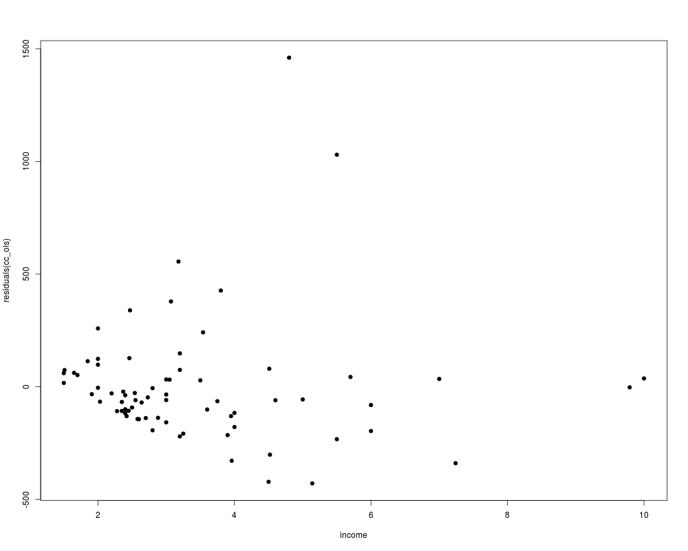
## Figure 11.1
plot(residuals(cc_ols) ~ income, data = ccard0, pch = 19)

## Table 11.1
mean(ccard$age)
prop.table(table(ccard$owner))
mean(ccard$income)

summary(cc_ols)
sqrt(diag(vcovHC(cc_ols, type = "HC0")))
sqrt(diag(vcovHC(cc_ols, type = "HC2"))) 
sqrt(diag(vcovHC(cc_ols, type = "HC1")))

bptest(cc_ols, ~ (age + income + I(income^2) + owner)^2 + I(age^2) + I(income^4), data = ccard0)
gqtest(cc_ols)
bptest(cc_ols, ~ income + I(income^2), data = ccard0, studentize = FALSE)
bptest(cc_ols, ~ income + I(income^2), data = ccard0)

## More examples can be found in:
## help("Greene2003")

Results


R version 3.3.1 (2016-06-21) -- "Bug in Your Hair"
Copyright (C) 2016 The R Foundation for Statistical Computing
Platform: x86_64-pc-linux-gnu (64-bit)

R is free software and comes with ABSOLUTELY NO WARRANTY.
You are welcome to redistribute it under certain conditions.
Type 'license()' or 'licence()' for distribution details.

R is a collaborative project with many contributors.
Type 'contributors()' for more information and
'citation()' on how to cite R or R packages in publications.

Type 'demo()' for some demos, 'help()' for on-line help, or
'help.start()' for an HTML browser interface to help.
Type 'q()' to quit R.

> library(AER)
Loading required package: car
Loading required package: lmtest
Loading required package: zoo

Attaching package: 'zoo'

The following objects are masked from 'package:base':

    as.Date, as.Date.numeric

Loading required package: sandwich
Loading required package: survival
> png(filename="/home/ddbj/snapshot/RGM3/R_CC/result/AER/CreditCard.Rd_%03d_medium.png", width=480, height=480)
> ### Name: CreditCard
> ### Title: Expenditure and Default Data
> ### Aliases: CreditCard
> ### Keywords: datasets
> 
> ### ** Examples
> 
> data("CreditCard")
> 
> ## Greene (2003)
> ## extract data set F9.1
> ccard <- CreditCard[1:100,]
> ccard$income <- round(ccard$income, digits = 2)
> ccard$expenditure <- round(ccard$expenditure, digits = 2)
> ccard$age <- round(ccard$age + .01)
> ## suspicious:
> CreditCard$age[CreditCard$age < 1]
[1] 0.5000000 0.1666667 0.5833333 0.7500000 0.5833333 0.5000000 0.7500000
> ## the first of these is also in TableF9.1 with 36 instead of 0.5:
> ccard$age[79] <- 36
> 
> ## Example 11.1
> ccard <- ccard[order(ccard$income),]
> ccard0 <- subset(ccard, expenditure > 0)
> cc_ols <- lm(expenditure ~ age + owner + income + I(income^2), data = ccard0)
> 
> ## Figure 11.1
> plot(residuals(cc_ols) ~ income, data = ccard0, pch = 19)
> 
> ## Table 11.1
> mean(ccard$age)
[1] 32.08
> prop.table(table(ccard$owner))

  no  yes 
0.64 0.36 
> mean(ccard$income)
[1] 3.3693
> 
> summary(cc_ols)

Call:
lm(formula = expenditure ~ age + owner + income + I(income^2), 
    data = ccard0)

Residuals:
    Min      1Q  Median      3Q     Max 
-429.00 -130.39  -51.89   53.96 1460.61 

Coefficients:
            Estimate Std. Error t value Pr(>|t|)   
(Intercept) -237.031    199.316  -1.189  0.23855   
age           -3.091      5.515  -0.560  0.57710   
owneryes      27.970     82.918   0.337  0.73693   
income       234.412     80.370   2.917  0.00481 **
I(income^2)  -15.002      7.469  -2.008  0.04863 * 
---
Signif. codes:  0 '***' 0.001 '**' 0.01 '*' 0.05 '.' 0.1 ' ' 1

Residual standard error: 284.7 on 67 degrees of freedom
Multiple R-squared:  0.2436,	Adjusted R-squared:  0.1985 
F-statistic: 5.395 on 4 and 67 DF,  p-value: 0.0007938

> sqrt(diag(vcovHC(cc_ols, type = "HC0")))
(Intercept)         age    owneryes      income I(income^2) 
 212.903038    3.300465   92.176017   88.864892    6.944454 
> sqrt(diag(vcovHC(cc_ols, type = "HC2"))) 
(Intercept)         age    owneryes      income I(income^2) 
 220.996881    3.446417   95.659360   92.082043    7.199455 
> sqrt(diag(vcovHC(cc_ols, type = "HC1")))
(Intercept)         age    owneryes      income I(income^2) 
 220.704255    3.421401   95.553541   92.121089    7.198913 
> 
> bptest(cc_ols, ~ (age + income + I(income^2) + owner)^2 + I(age^2) + I(income^4), data = ccard0)

	studentized Breusch-Pagan test

data:  cc_ols
BP = 14.327, df = 12, p-value = 0.2803

> gqtest(cc_ols)

	Goldfeld-Quandt test

data:  cc_ols
GQ = 15.006, df1 = 31, df2 = 31, p-value = 1.372e-11

> bptest(cc_ols, ~ income + I(income^2), data = ccard0, studentize = FALSE)

	Breusch-Pagan test

data:  cc_ols
BP = 41.921, df = 2, p-value = 7.889e-10

> bptest(cc_ols, ~ income + I(income^2), data = ccard0)

	studentized Breusch-Pagan test

data:  cc_ols
BP = 6.1863, df = 2, p-value = 0.04536

> 
> ## More examples can be found in:
> ## help("Greene2003")
> 
> 
> 
> 
> 
> dev.off()
null device 
          1 
>