German Socio-Economic Panel 1994–2002

Description

Cross-section data for 675 14-year old children born between 1980 and 1988. The sample is taken from the German Socio-Economic Panel (GSOEP) for the years 1994 to 2002 to investigate the determinants of secondary school choice.

Usage

data("GSOEP9402")

Format

A data frame containing 675 observations on 12 variables.

school

factor. Child's secondary school level.

birthyear

Year of child's birth.

gender

factor indicating child's gender.

kids

Total number of kids living in household.

parity

Birth order.

income

Household income.

size

Household size

state

factor indicating German federal state.

marital

factor indicating mother's marital status.

meducation

Mother's educational level in years.

memployment

factor indicating mother's employment level: full-time, part-time, or not working.

year

Year of GSOEP wave.

Details

This sample from the German Socio-Economic Panel (GSOEP) for the years between 1994 and 2002 has been selected by Winkelmann and Boes (2009) to investigate the determinants of secondary school choice.

In the German schooling system, students are separated relatively early into different school types, depending on their ability as perceived by the teachers after four years of primary school. After that, around the age of ten, students are placed into one of three types of secondary school: "Hauptschule" (lower secondary school), "Realschule" (middle secondary school), or "Gymnasium" (upper secondary school). Only a degree from the latter type of school (called Abitur) provides direct access to universities.

A frequent criticism of this system is that the tracking takes place too early, and that it cements inequalities in education across generations. Although the secondary school choice is based on the teachers' recommendations, it is typically also influenced by the parents; both indirectly through their own educational level and directly through influence on the teachers.

Source

Online complements to Winkelmann and Boes (2009).

http://www.econ.uzh.ch/faculty/groupwinkelmann/research/publications/microdata/datasets/school.zip

References

Winkelmann, R., and Boes, S. (2009). Analysis of Microdata, 2nd ed. Berlin and Heidelberg: Springer-Verlag.

See Also

WinkelmannBoes2009

Examples

## data
data("GSOEP9402", package = "AER")

## some convenience data transformations
gsoep <- GSOEP9402
gsoep$year2 <- factor(gsoep$year)

## visualization
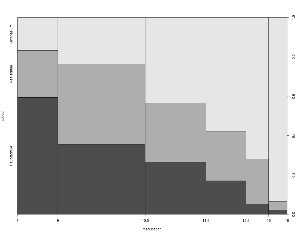
plot(school ~ meducation, data = gsoep, breaks = c(7, 9, 10.5, 11.5, 12.5, 15, 18))


## Chapter 5, Table 5.1
library("nnet")
gsoep_mnl <- multinom(
  school ~ meducation + memployment + log(income) + log(size) + parity + year2,
  data = gsoep)
coeftest(gsoep_mnl)[c(1:6, 1:6 + 14),]
 
## alternatively
if(require("mlogit")) {
gsoep_mnl2 <- mlogit(
  school ~ 0 | meducation + memployment + log(income) + log(size) + parity + year2,
  data = gsoep, shape = "wide", reflevel = "Hauptschule")
coeftest(gsoep_mnl2)[1:12,]
}

## Table 5.2
library("effects")
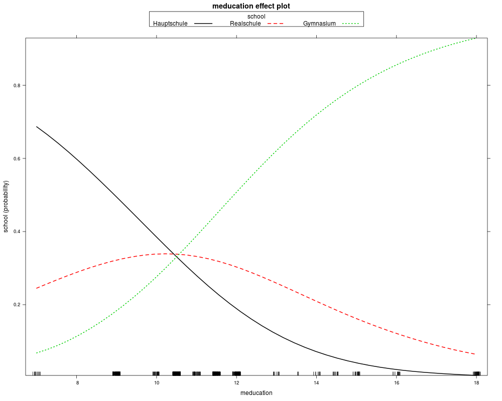
gsoep_eff <- effect("meducation", gsoep_mnl,
  xlevels = list(meducation = sort(unique(gsoep$meducation))))
gsoep_eff$prob
plot(gsoep_eff, confint = FALSE)

## omit year
gsoep_mnl1 <- multinom(
  school ~ meducation + memployment + log(income) + log(size) + parity,
  data = gsoep)
lrtest(gsoep_mnl, gsoep_mnl1)


## Chapter 6
## Table 6.1
library("MASS")
gsoep_pop <- polr(
  school ~ meducation + I(memployment != "none") + log(income) + log(size) + parity + year2,
  data = gsoep, method = "probit", Hess = TRUE)
gsoep_pol <- polr(
  school ~ meducation + I(memployment != "none") + log(income) + log(size) + parity + year2,
  data = gsoep, Hess = TRUE)

## compare polr and multinom via AIC
gsoep_pol1 <- polr(
  school ~ meducation + memployment + log(income) + log(size) + parity,
  data = gsoep, Hess = TRUE)
AIC(gsoep_pol1, gsoep_mnl)

## effects
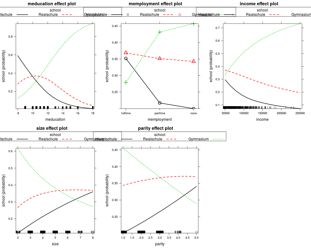
eff_pol1 <- allEffects(gsoep_pol1)
plot(eff_pol1, ask = FALSE, confint = FALSE)


## More examples can be found in:
## help("WinkelmannBoes2009")

Results

R version 3.3.1 (2016-06-21) -- "Bug in Your Hair"
Copyright (C) 2016 The R Foundation for Statistical Computing
Platform: x86_64-pc-linux-gnu (64-bit)

R is free software and comes with ABSOLUTELY NO WARRANTY.
You are welcome to redistribute it under certain conditions.
Type 'license()' or 'licence()' for distribution details.

R is a collaborative project with many contributors.
Type 'contributors()' for more information and
'citation()' on how to cite R or R packages in publications.

Type 'demo()' for some demos, 'help()' for on-line help, or
'help.start()' for an HTML browser interface to help.
Type 'q()' to quit R.

> library(AER)
Loading required package: car
Loading required package: lmtest
Loading required package: zoo

Attaching package: 'zoo'

The following objects are masked from 'package:base':

    as.Date, as.Date.numeric

Loading required package: sandwich
Loading required package: survival
> png(filename="/home/ddbj/snapshot/RGM3/R_CC/result/AER/GSOEP9402.Rd_%03d_medium.png", width=480, height=480)
> ### Name: GSOEP9402
> ### Title: German Socio-Economic Panel 1994-2002
> ### Aliases: GSOEP9402
> ### Keywords: datasets
> 
> ### ** Examples
> 
> ## data
> data("GSOEP9402", package = "AER")
> 
> ## some convenience data transformations
> gsoep <- GSOEP9402
> gsoep$year2 <- factor(gsoep$year)
> 
> ## visualization
> plot(school ~ meducation, data = gsoep, breaks = c(7, 9, 10.5, 11.5, 12.5, 15, 18))
> 
> 
> ## Chapter 5, Table 5.1
> library("nnet")
> gsoep_mnl <- multinom(
+   school ~ meducation + memployment + log(income) + log(size) + parity + year2,
+   data = gsoep)
# weights:  48 (30 variable)
initial  value 741.563295 
iter  10 value 655.748279
iter  20 value 624.992858
iter  30 value 618.605354
final  value 618.475696 
converged
> coeftest(gsoep_mnl)[c(1:6, 1:6 + 14),]
                                  Estimate Std. Error    z value     Pr(>|z|)
Realschule:(Intercept)          -6.3864877 2.36903996 -2.6958126 7.021716e-03
Realschule:meducation            0.3004843 0.07910641  3.7984819 1.455851e-04
Realschule:memploymentparttime   0.4933680 0.32189721  1.5326879 1.253528e-01
Realschule:memploymentnone       0.7526399 0.32884476  2.2887392 2.209451e-02
Realschule:log(income)           0.3934871 0.22539836  1.7457408 8.085601e-02
Realschule:log(size)            -1.1921790 0.44641156 -2.6705827 7.571972e-03
Realschule:year22002             0.1922413 0.45158350  0.4257049 6.703229e-01
Gymnasium:(Intercept)          -23.6975758 3.01022807 -7.8723523 3.480345e-15
Gymnasium:meducation             0.6597649 0.08144034  8.1012060 5.441700e-16
Gymnasium:memploymentparttime    0.9372429 0.34536421  2.7137813 6.652007e-03
Gymnasium:memploymentnone        1.1007579 0.35842760  3.0710746 2.132898e-03
Gymnasium:log(income)            1.6676745 0.28408439  5.8703492 4.348783e-09
>  
> ## alternatively
> if(require("mlogit")) {
+ gsoep_mnl2 <- mlogit(
+   school ~ 0 | meducation + memployment + log(income) + log(size) + parity + year2,
+   data = gsoep, shape = "wide", reflevel = "Hauptschule")
+ coeftest(gsoep_mnl2)[1:12,]
+ }
Loading required package: mlogit
Loading required package: Formula
Loading required package: maxLik
Loading required package: miscTools

Please cite the 'maxLik' package as:
Henningsen, Arne and Toomet, Ott (2011). maxLik: A package for maximum likelihood estimation in R. Computational Statistics 26(3), 443-458. DOI 10.1007/s00180-010-0217-1.

If you have questions, suggestions, or comments regarding the 'maxLik' package, please use a forum or 'tracker' at maxLik's R-Forge site:
https://r-forge.r-project.org/projects/maxlik/
                                  Estimate Std. Error   t value     Pr(>|t|)
Gymnasium:(intercept)          -23.6982768 3.01026604 -7.872486 1.475202e-14
Realschule:(intercept)          -6.3865987 2.36904833 -2.695850 7.204061e-03
Gymnasium:meducation             0.6597829 0.08144157  8.101304 2.726719e-15
Realschule:meducation            0.3004923 0.07910725  3.798543 1.593085e-04
Gymnasium:memploymentparttime    0.9372401 0.34536576  2.713761 6.830145e-03
Realschule:memploymentparttime   0.4933644 0.32189760  1.532675 1.258463e-01
Gymnasium:memploymentnone        1.1007670 0.35842942  3.071084 2.222541e-03
Realschule:memploymentnone       0.7526490 0.32884523  2.288764 2.241551e-02
Gymnasium:log(income)            1.6677258 0.28408738  5.870468 6.954975e-09
Realschule:log(income)           0.3934899 0.22539876  1.745750 8.133056e-02
Gymnasium:log(size)             -1.5459256 0.48775919 -3.169444 1.599570e-03
Realschule:log(size)            -1.1921835 0.44641174 -2.670592 7.762668e-03
> 
> ## Table 5.2
> library("effects")

Attaching package: 'effects'

The following object is masked from 'package:car':

    Prestige

> gsoep_eff <- effect("meducation", gsoep_mnl,
+   xlevels = list(meducation = sort(unique(gsoep$meducation))))
> gsoep_eff$prob
      prob.Hauptschule prob.Realschule prob.Gymnasium
 [1,]      0.686724467      0.24514452     0.06813102
 [2,]      0.494486442      0.32195219     0.18356137
 [3,]      0.385007121      0.33853566     0.27645721
 [4,]      0.331068546      0.33830072     0.33063074
 [5,]      0.279605513      0.33203209     0.38836239
 [6,]      0.231922018      0.32005576     0.44802222
 [7,]      0.189019319      0.30313717     0.50784351
 [8,]      0.119575666      0.25898492     0.62143941
 [9,]      0.093066080      0.23424613     0.67268779
[10,]      0.071541719      0.20926168     0.71919660
[11,]      0.054404764      0.18493393     0.76066131
[12,]      0.040990572      0.16192466     0.79708477
[13,]      0.022753542      0.12138826     0.85585820
[14,]      0.006601958      0.06423885     0.92915919
> plot(gsoep_eff, confint = FALSE)
> 
> ## omit year
> gsoep_mnl1 <- multinom(
+   school ~ meducation + memployment + log(income) + log(size) + parity,
+   data = gsoep)
# weights:  24 (14 variable)
initial  value 741.563295 
iter  10 value 658.442291
iter  20 value 624.980518
final  value 624.957624 
converged
> lrtest(gsoep_mnl, gsoep_mnl1)
Likelihood ratio test

Model 1: school ~ meducation + memployment + log(income) + log(size) + 
    parity + year2
Model 2: school ~ meducation + memployment + log(income) + log(size) + 
    parity
  #Df  LogLik  Df  Chisq Pr(>Chisq)
1  30 -618.48                      
2  14 -624.96 -16 12.964     0.6754
> 
> 
> ## Chapter 6
> ## Table 6.1
> library("MASS")
> gsoep_pop <- polr(
+   school ~ meducation + I(memployment != "none") + log(income) + log(size) + parity + year2,
+   data = gsoep, method = "probit", Hess = TRUE)
> gsoep_pol <- polr(
+   school ~ meducation + I(memployment != "none") + log(income) + log(size) + parity + year2,
+   data = gsoep, Hess = TRUE)
> 
> ## compare polr and multinom via AIC
> gsoep_pol1 <- polr(
+   school ~ meducation + memployment + log(income) + log(size) + parity,
+   data = gsoep, Hess = TRUE)
> AIC(gsoep_pol1, gsoep_mnl)
           df      AIC
gsoep_pol1  8 1275.075
gsoep_mnl  30 1296.951
> 
> ## effects
> eff_pol1 <- allEffects(gsoep_pol1)
> plot(eff_pol1, ask = FALSE, confint = FALSE)
> 
> 
> ## More examples can be found in:
> ## help("WinkelmannBoes2009")
> 
> 
> 
> 
> 
> dev.off()
null device 
          1 
>