Data and Examples from Greene (2003)

Description

This manual page collects a list of examples from the book. Some solutions might not be exact and the list is certainly not complete. If you have suggestions for improvement (preferably in the form of code), please contact the package maintainer.

References

Greene, W.H. (2003). Econometric Analysis, 5th edition. Upper Saddle River, NJ: Prentice Hall. URL http://pages.stern.nyu.edu/~wgreene/Text/tables/tablelist5.htm.

See Also

Affairs, BondYield, CreditCard, Electricity1955, Electricity1970, Equipment, Grunfeld, KleinI, Longley, ManufactCosts, MarkPound, Municipalities, ProgramEffectiveness, PSID1976, SIC33, ShipAccidents, StrikeDuration, TechChange, TravelMode, UKInflation, USConsump1950, USConsump1979, USGasG, USAirlines, USInvest, USMacroG, USMoney

Examples

#####################################
## US consumption data (1970-1979) ##
#####################################

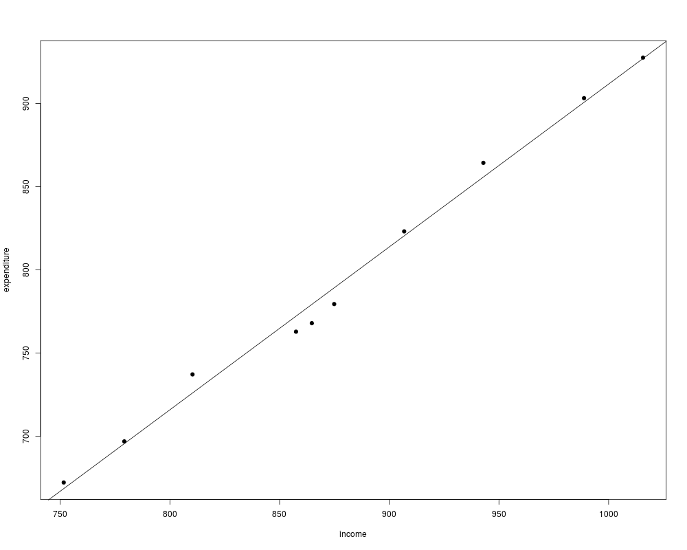
## Example 1.1
data("USConsump1979", package = "AER")
plot(expenditure ~ income, data = as.data.frame(USConsump1979), pch = 19)
fm <- lm(expenditure ~ income, data = as.data.frame(USConsump1979))
summary(fm)
abline(fm)


#####################################
## US consumption data (1940-1950) ##
#####################################

## data
data("USConsump1950", package = "AER")
usc <- as.data.frame(USConsump1950)
usc$war <- factor(usc$war, labels = c("no", "yes"))

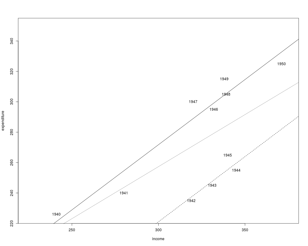
## Example 2.1
plot(expenditure ~ income, data = usc, type = "n", xlim = c(225, 375), ylim = c(225, 350))
with(usc, text(income, expenditure, time(USConsump1950)))

## single model
fm <- lm(expenditure ~ income, data = usc)
summary(fm)

## different intercepts for war yes/no
fm2 <- lm(expenditure ~ income + war, data = usc)
summary(fm2)

## compare
anova(fm, fm2)

## visualize
abline(fm, lty = 3)                                   
abline(coef(fm2)[1:2])                                
abline(sum(coef(fm2)[c(1, 3)]), coef(fm2)[2], lty = 2)

## Example 3.2
summary(fm)$r.squared
summary(lm(expenditure ~ income, data = usc, subset = war == "no"))$r.squared
summary(fm2)$r.squared


########################
## US investment data ##
########################

data("USInvest", package = "AER")

## Chapter 3 in Greene (2003)
## transform (and round) data to match Table 3.1
us <- as.data.frame(USInvest)
us$invest <- round(0.1 * us$invest/us$price, digits = 3)
us$gnp <- round(0.1 * us$gnp/us$price, digits = 3)
us$inflation <- c(4.4, round(100 * diff(us$price)/us$price[-15], digits = 2))
us$trend <- 1:15
us <- us[, c(2, 6, 1, 4, 5)]

## p. 22-24
coef(lm(invest ~ trend + gnp, data = us))
coef(lm(invest ~ gnp, data = us))

## Example 3.1, Table 3.2
cor(us)[1,-1]
pcor <- solve(cor(us))
dcor <- 1/sqrt(diag(pcor))
pcor <- (-pcor * (dcor %o% dcor))[1,-1]

## Table 3.4
fm  <- lm(invest ~ trend + gnp + interest + inflation, data = us)
fm1 <- lm(invest ~ 1, data = us)
anova(fm1, fm)

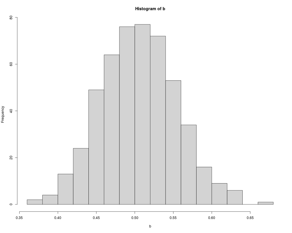
## Example 4.1
set.seed(123)
w <- rnorm(10000)
x <- rnorm(10000)
eps <- 0.5 * w
y <- 0.5 + 0.5 * x + eps
b <- rep(0, 500)
for(i in 1:500) {
  ix <- sample(1:10000, 100)
  b[i] <- lm.fit(cbind(1, x[ix]), y[ix])$coef[2]
}
hist(b, breaks = 20, col = "lightgray")


###############################
## Longley's regression data ##
###############################

## package and data
data("Longley", package = "AER")
library("dynlm")

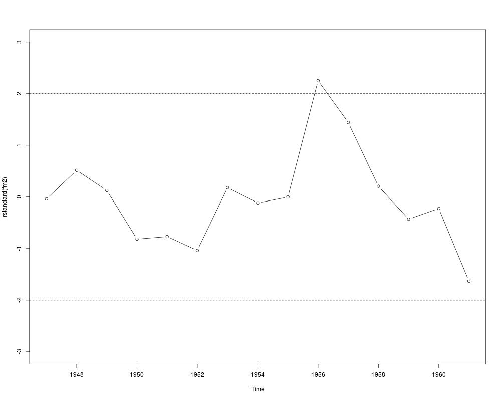
## Example 4.6
fm1 <- dynlm(employment ~ time(employment) + price + gnp + armedforces,
  data = Longley)
fm2 <- update(fm1, end = 1961)
cbind(coef(fm2), coef(fm1))

## Figure 4.3
plot(rstandard(fm2), type = "b", ylim = c(-3, 3))
abline(h = c(-2, 2), lty = 2)


#########################################
## US gasoline market data (1960-1995) ##
#########################################

## data
data("USGasG", package = "AER")

## Greene (2003)
## Example 2.3
fm <- lm(log(gas/population) ~ log(price) + log(income) + log(newcar) + log(usedcar),
  data = as.data.frame(USGasG))
summary(fm)

## Example 4.4
## estimates and standard errors (note different offset for intercept)
coef(fm)
sqrt(diag(vcov(fm)))
## confidence interval
confint(fm, parm = "log(income)")
## test linear hypothesis
linearHypothesis(fm, "log(income) = 1")

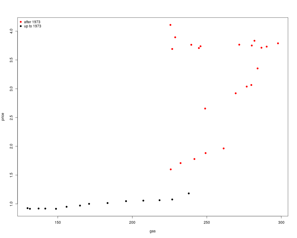
## Figure 7.5
plot(price ~ gas, data = as.data.frame(USGasG), pch = 19,
  col = (time(USGasG) > 1973) + 1)
legend("topleft", legend = c("after 1973", "up to 1973"), pch = 19, col = 2:1, bty = "n")

## Example 7.6
## re-used in Example 8.3
## linear time trend
ltrend <- 1:nrow(USGasG)
## shock factor
shock <- factor(time(USGasG) > 1973, levels = c(FALSE, TRUE), labels = c("before", "after"))

## 1960-1995
fm1 <- lm(log(gas/population) ~ log(income) + log(price) + log(newcar) + log(usedcar) + ltrend,
  data = as.data.frame(USGasG))
summary(fm1)
## pooled
fm2 <- lm(
  log(gas/population) ~ shock + log(income) + log(price) + log(newcar) + log(usedcar) + ltrend,
  data = as.data.frame(USGasG))
summary(fm2)
## segmented
fm3 <- lm(
  log(gas/population) ~ shock/(log(income) + log(price) + log(newcar) + log(usedcar) + ltrend),
  data = as.data.frame(USGasG))
summary(fm3)

## Chow test
anova(fm3, fm1)
library("strucchange")
sctest(log(gas/population) ~ log(income) + log(price) + log(newcar) + log(usedcar) + ltrend,
  data = USGasG, point = c(1973, 1), type = "Chow")
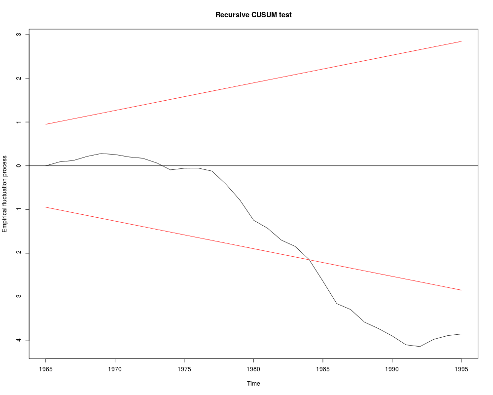
## Recursive CUSUM test
rcus <- efp(log(gas/population) ~ log(income) + log(price) + log(newcar) + log(usedcar) + ltrend,
   data = USGasG, type = "Rec-CUSUM")
plot(rcus)
sctest(rcus)
## Note: Greene's remark that the break is in 1984 (where the process crosses its boundary)
## is wrong. The break appears to be no later than 1976.

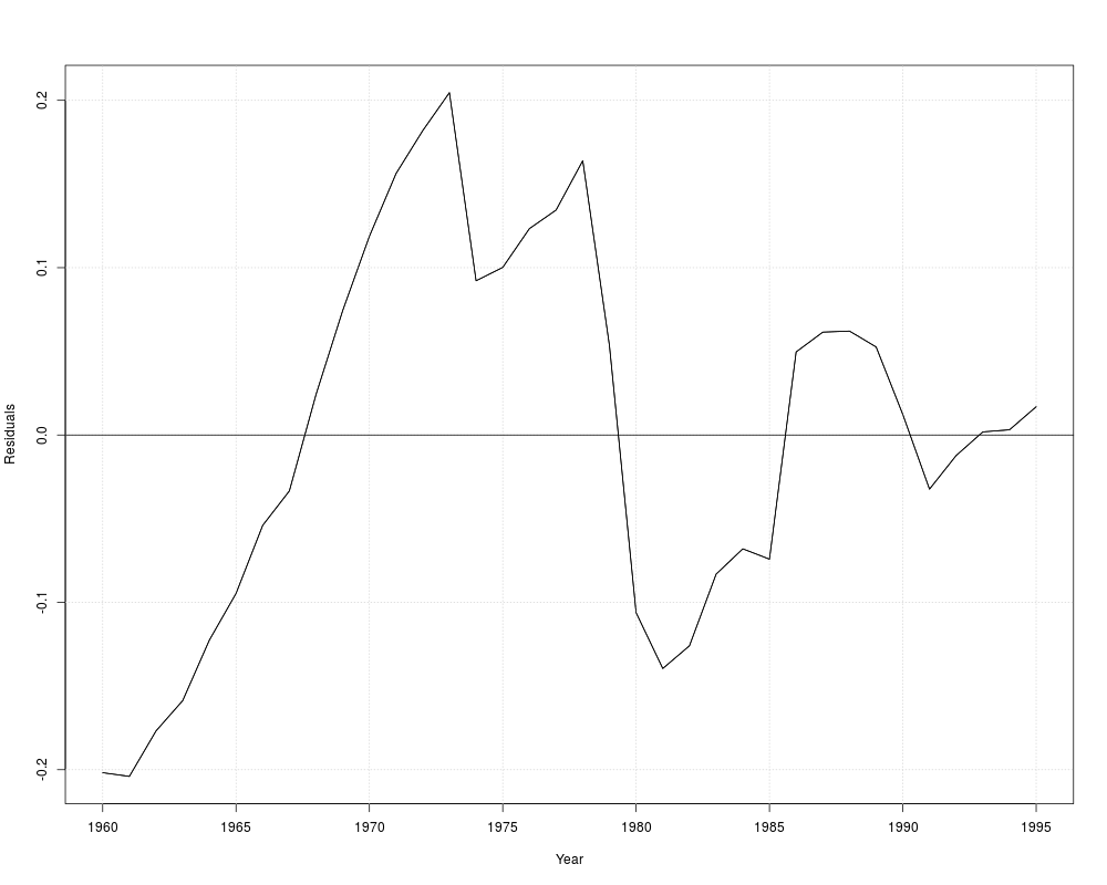
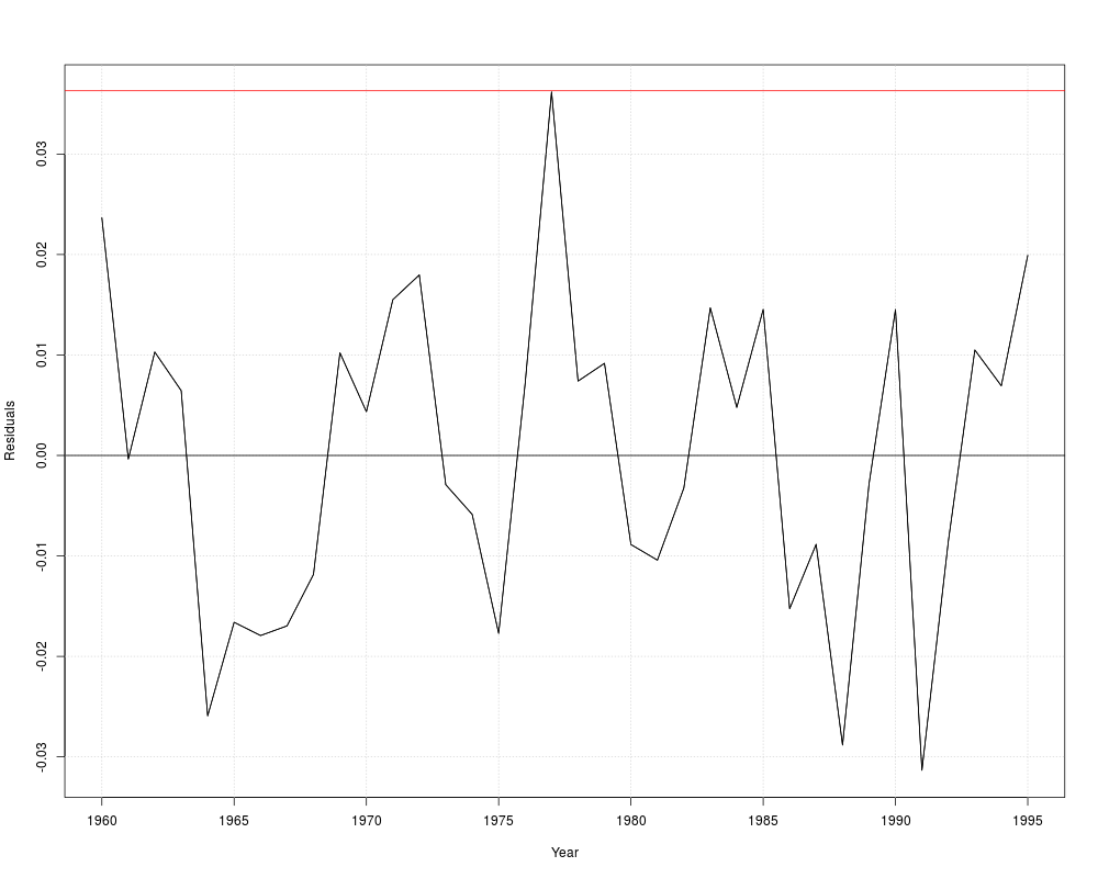
## Example 12.2
library("dynlm")
resplot <- function(obj, bound = TRUE) {
  res <- residuals(obj)
  sigma <- summary(obj)$sigma
  plot(res, ylab = "Residuals", xlab = "Year")
  grid()
  abline(h = 0)
  if(bound) abline(h = c(-2, 2) * sigma, col = "red")  
  lines(res)
}
resplot(dynlm(log(gas/population) ~ log(price), data = USGasG))
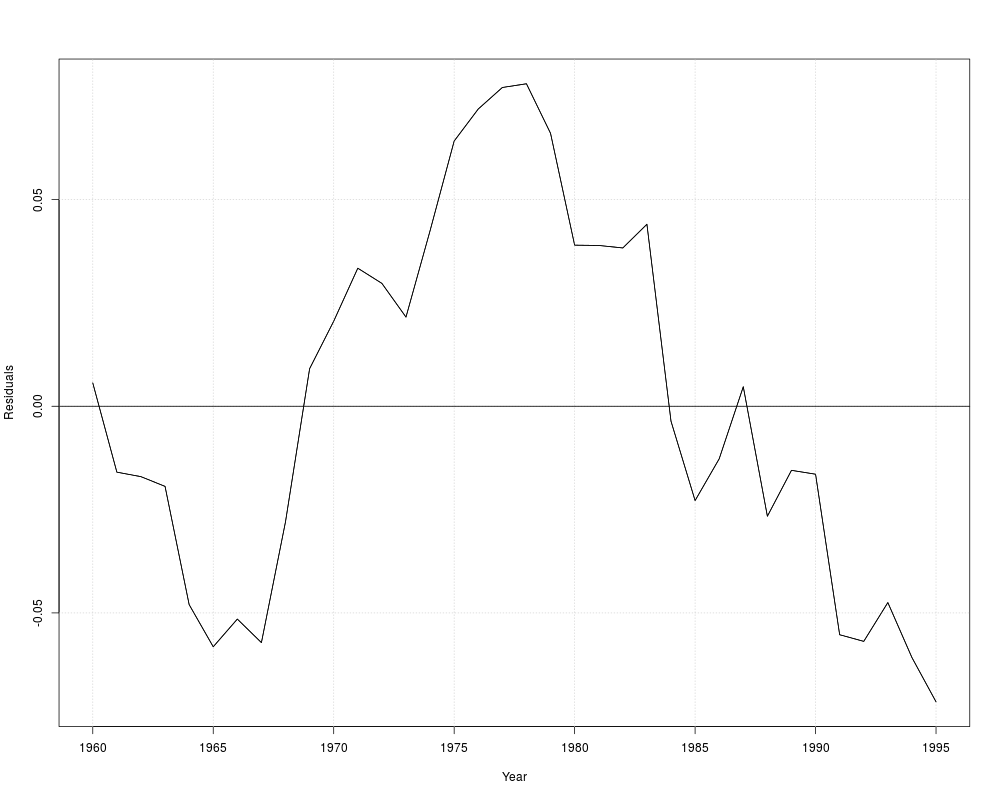
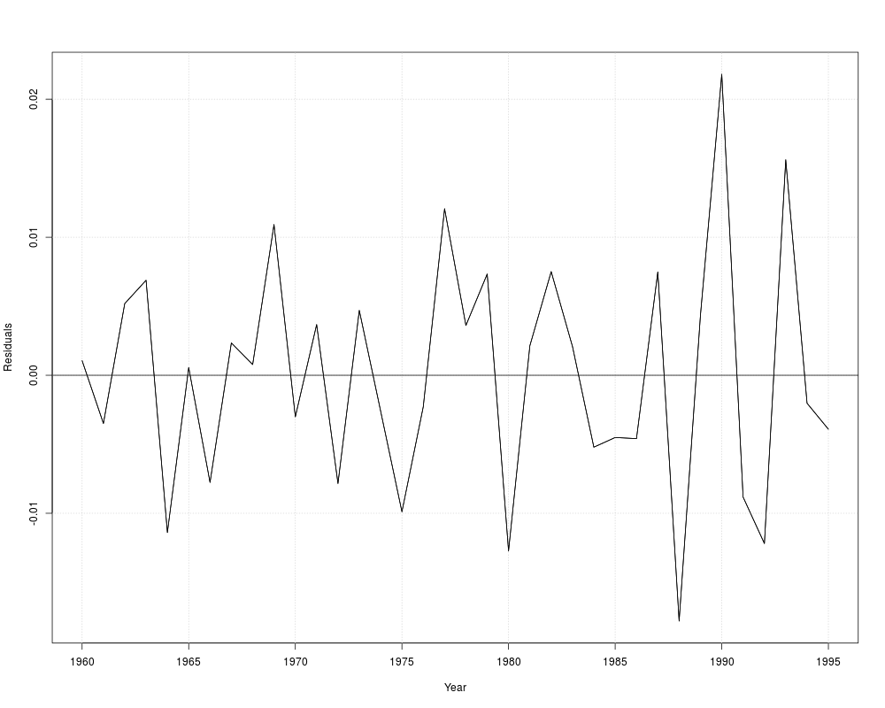
resplot(dynlm(log(gas/population) ~ log(price) + log(income), data = USGasG))
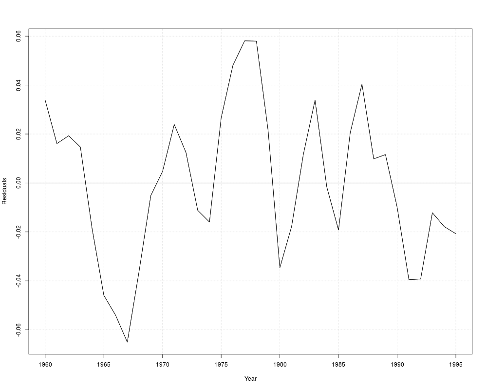
resplot(dynlm(log(gas/population) ~ log(price) + log(income) + log(newcar) + log(usedcar) +
  log(transport) + log(nondurable) + log(durable) +log(service) + ltrend, data = USGasG))
## different shock variable than in 7.6
shock <- factor(time(USGasG) > 1974, levels = c(FALSE, TRUE), labels = c("before", "after"))
resplot(dynlm(log(gas/population) ~ shock/(log(price) + log(income) + log(newcar) + log(usedcar) +
  log(transport) + log(nondurable) + log(durable) + log(service) + ltrend), data = USGasG))
## NOTE: something seems to be wrong with the sigma estimates in the `full' models

## Table 12.4, OLS
fm <- dynlm(log(gas/population) ~ log(price) + log(income) + log(newcar) + log(usedcar),
  data = USGasG)
summary(fm)
resplot(fm, bound = FALSE)
dwtest(fm)

## ML
g <- as.data.frame(USGasG)
y <- log(g$gas/g$population)
X <- as.matrix(cbind(log(g$price), log(g$income), log(g$newcar), log(g$usedcar)))
arima(y, order = c(1, 0, 0), xreg = X)


#######################################
## US macroeconomic data (1950-2000) ##
#######################################
## data and trend
data("USMacroG", package = "AER")
ltrend <- 0:(nrow(USMacroG) - 1)

## Example 5.3
## OLS and IV regression
library("dynlm")
fm_ols <- dynlm(consumption ~ gdp, data = USMacroG)
fm_iv <- dynlm(consumption ~ gdp | L(consumption) + L(gdp), data = USMacroG)

## Hausman statistic
library("MASS")
b_diff <- coef(fm_iv) - coef(fm_ols)
v_diff <- summary(fm_iv)$cov.unscaled - summary(fm_ols)$cov.unscaled
(t(b_diff) %*% ginv(v_diff) %*% b_diff) / summary(fm_ols)$sigma^2

## Wu statistic
auxreg <- dynlm(gdp ~ L(consumption) + L(gdp), data = USMacroG)
coeftest(dynlm(consumption ~ gdp + fitted(auxreg), data = USMacroG))[3,3] 
## agrees with Greene (but not with errata)

## Example 6.1
## Table 6.1
fm6.1 <- dynlm(log(invest) ~ tbill + inflation + log(gdp) + ltrend, data = USMacroG)
fm6.3 <- dynlm(log(invest) ~ I(tbill - inflation) + log(gdp) + ltrend, data = USMacroG)
summary(fm6.1)
summary(fm6.3)
deviance(fm6.1)
deviance(fm6.3)
vcov(fm6.1)[2,3] 

## F test
linearHypothesis(fm6.1, "tbill + inflation = 0")
## alternatively
anova(fm6.1, fm6.3)
## t statistic
sqrt(anova(fm6.1, fm6.3)[2,5])
 
## Example 6.3
## Distributed lag model:
## log(Ct) = b0 + b1 * log(Yt) + b2 * log(C(t-1)) + u
us <- log(USMacroG[, c(2, 5)])
fm_distlag <- dynlm(log(consumption) ~ log(dpi) + L(log(consumption)),
  data = USMacroG)
summary(fm_distlag)

## estimate and test long-run MPC 
coef(fm_distlag)[2]/(1-coef(fm_distlag)[3])
linearHypothesis(fm_distlag, "log(dpi) + L(log(consumption)) = 1")
## correct, see errata
 
## Example 6.4
## predict investiment in 2001(1)
predict(fm6.1, interval = "prediction",
  newdata = data.frame(tbill = 4.48, inflation = 5.262, gdp = 9316.8, ltrend = 204))

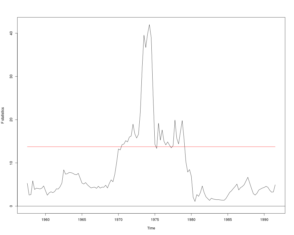
## Example 7.7
## no GMM available in "strucchange"
## using OLS instead yields
fs <- Fstats(log(m1/cpi) ~ log(gdp) + tbill, data = USMacroG,
  vcov = NeweyWest, from = c(1957, 3), to = c(1991, 3))
plot(fs)
## which looks somewhat similar ...
 
## Example 8.2
## Ct = b0 + b1*Yt + b2*Y(t-1) + v
fm1 <- dynlm(consumption ~ dpi + L(dpi), data = USMacroG)
## Ct = a0 + a1*Yt + a2*C(t-1) + u
fm2 <- dynlm(consumption ~ dpi + L(consumption), data = USMacroG)

## Cox test in both directions:
coxtest(fm1, fm2)
## ... and do the same for jtest() and encomptest().
## Notice that in this particular case two of them are coincident.
jtest(fm1, fm2)
encomptest(fm1, fm2)
## encomptest could also be performed `by hand' via
fmE <- dynlm(consumption ~ dpi + L(dpi) + L(consumption), data = USMacroG)
waldtest(fm1, fmE, fm2)

## Table 9.1
fm_ols <- lm(consumption ~ dpi, data = as.data.frame(USMacroG))
fm_nls <- nls(consumption ~ alpha + beta * dpi^gamma,
  start = list(alpha = coef(fm_ols)[1], beta = coef(fm_ols)[2], gamma = 1),
  control = nls.control(maxiter = 100), data = as.data.frame(USMacroG))
summary(fm_ols)
summary(fm_nls)
deviance(fm_ols)
deviance(fm_nls)
vcov(fm_nls)

## Example 9.7
## F test
fm_nls2 <- nls(consumption ~ alpha + beta * dpi,
  start = list(alpha = coef(fm_ols)[1], beta = coef(fm_ols)[2]),
  control = nls.control(maxiter = 100), data = as.data.frame(USMacroG))
anova(fm_nls, fm_nls2)
## Wald test
linearHypothesis(fm_nls, "gamma = 1")

## Example 9.8, Table 9.2
usm <- USMacroG[, c("m1", "tbill", "gdp")]
fm_lin <- lm(m1 ~ tbill + gdp, data = usm)
fm_log <- lm(m1 ~ tbill + gdp, data = log(usm))
## PE auxiliary regressions
aux_lin <- lm(m1 ~ tbill + gdp + I(fitted(fm_log) - log(fitted(fm_lin))), data = usm)
aux_log <- lm(m1 ~ tbill + gdp + I(fitted(fm_lin) - exp(fitted(fm_log))), data = log(usm))
coeftest(aux_lin)[4,]
coeftest(aux_log)[4,]
## matches results from errata
## With lmtest >= 0.9-24:
## petest(fm_lin, fm_log)

## Example 12.1
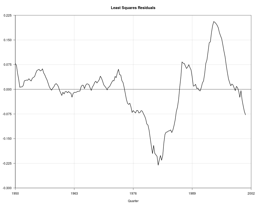
fm_m1 <- dynlm(log(m1) ~ log(gdp) + log(cpi), data = USMacroG)
summary(fm_m1)

## Figure 12.1
par(las = 1)
plot(0, 0, type = "n", axes = FALSE,
     xlim = c(1950, 2002), ylim = c(-0.3, 0.225),
     xaxs = "i", yaxs = "i",
     xlab = "Quarter", ylab = "", main = "Least Squares Residuals")
box()
axis(1, at = c(1950, 1963, 1976, 1989, 2002))
axis(2, seq(-0.3, 0.225, by = 0.075))
grid(4, 7, col = grey(0.6))
abline(0, 0)
lines(residuals(fm_m1), lwd = 2)

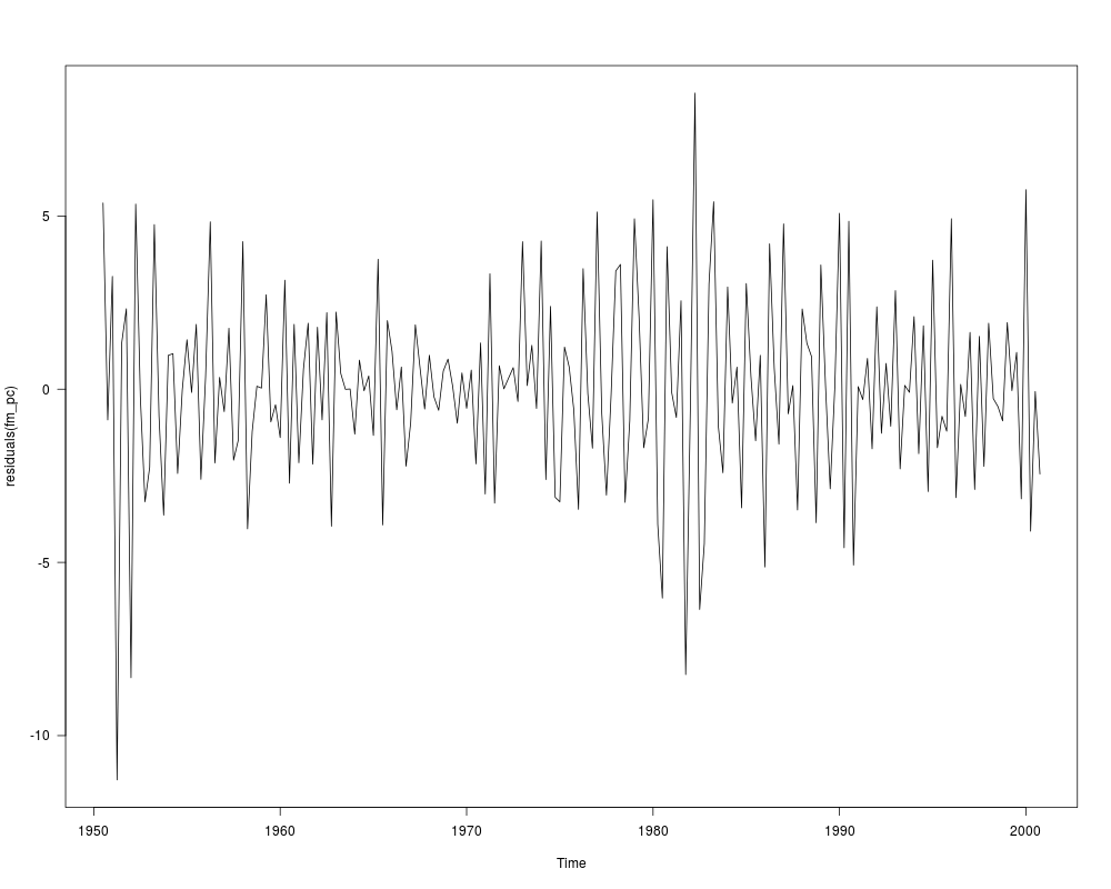
## Example 12.3
fm_pc <- dynlm(d(inflation) ~ unemp, data = USMacroG)
summary(fm_pc)
## Figure 12.3
plot(residuals(fm_pc))
## natural unemployment rate
coef(fm_pc)[1]/coef(fm_pc)[2]
## autocorrelation
res <- residuals(fm_pc)
summary(dynlm(res ~ L(res)))

## Example 12.4
coeftest(fm_m1)
coeftest(fm_m1, vcov = NeweyWest(fm_m1, lag = 5))
summary(fm_m1)$r.squared
dwtest(fm_m1)
as.vector(acf(residuals(fm_m1), plot = FALSE)$acf)[2]
## matches Tab. 12.1 errata and Greene 6e, apart from Newey-West SE


#################################################
## Cost function of electricity producers 1870 ##
#################################################

## Example 5.6: a generalized Cobb-Douglas cost function
data("Electricity1970", package = "AER")
fm <- lm(log(cost/fuel) ~ log(output) + I(log(output)^2/2) + 
  log(capital/fuel) + log(labor/fuel), data=Electricity1970[1:123,])


####################################################
## SIC 33: Production for primary metals industry ##
####################################################

## data
data("SIC33", package = "AER")

## Example 6.2
## Translog model
fm_tl <- lm(
  output ~ labor + capital + I(0.5 * labor^2) + I(0.5 * capital^2) + I(labor * capital),
  data = log(SIC33))
## Cobb-Douglas model
fm_cb <- lm(output ~ labor + capital, data = log(SIC33))

## Table 6.2 in Greene (2003)
deviance(fm_tl)
deviance(fm_cb)
summary(fm_tl)
summary(fm_cb)
vcov(fm_tl)
vcov(fm_cb)

## Cobb-Douglas vs. Translog model
anova(fm_cb, fm_tl)
## hypothesis of constant returns
linearHypothesis(fm_cb, "labor + capital = 1")


###############################
## Cost data for US airlines ##
###############################

## data
data("USAirlines", package = "AER")

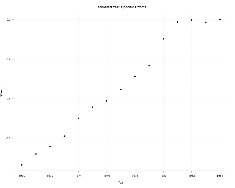
## Example 7.2
fm_full <- lm(log(cost) ~ log(output) + I(log(output)^2) + log(price) + load + year + firm,
  data = USAirlines)
fm_time <- lm(log(cost) ~ log(output) + I(log(output)^2) + log(price) + load + year,
  data = USAirlines)
fm_firm <- lm(log(cost) ~ log(output) + I(log(output)^2) + log(price) + load + firm,
  data = USAirlines)
fm_no <- lm(log(cost) ~ log(output) + I(log(output)^2) + log(price) + load, data = USAirlines)

## full fitted model
coef(fm_full)[1:5]
plot(1970:1984, c(coef(fm_full)[6:19], 0), type = "n",
     xlab = "Year", ylab = expression(delta(Year)),
     main = "Estimated Year Specific Effects")
grid()
points(1970:1984, c(coef(fm_full)[6:19], 0), pch = 19)

## Table 7.2
anova(fm_full, fm_time)
anova(fm_full, fm_firm)
anova(fm_full, fm_no)

## alternatively, use plm()
library("plm")
usair <- plm.data(USAirlines, c("firm", "year"))
fm_full2 <- plm(log(cost) ~ log(output) + I(log(output)^2) + log(price) + load,
  data = usair, model = "within", effect = "twoways")
fm_time2 <- plm(log(cost) ~ log(output) + I(log(output)^2) + log(price) + load,
  data = usair, model = "within", effect = "time")
fm_firm2 <- plm(log(cost) ~ log(output) + I(log(output)^2) + log(price) + load,
  data = usair, model = "within", effect = "individual")
fm_no2 <- plm(log(cost) ~ log(output) + I(log(output)^2) + log(price) + load,
  data = usair, model = "pooling")
pFtest(fm_full2, fm_time2)
pFtest(fm_full2, fm_firm2)
pFtest(fm_full2, fm_no2)


## Example 13.1, Table 13.1
fm_no <- plm(log(cost) ~ log(output) + log(price) + load, data = usair, model = "pooling")
fm_gm <- plm(log(cost) ~ log(output) + log(price) + load, data = usair, model = "between")
fm_firm <- plm(log(cost) ~ log(output) + log(price) + load, data = usair, model = "within")
fm_time <- plm(log(cost) ~ log(output) + log(price) + load, data = usair, model = "within",
  effect = "time")
fm_ft <- plm(log(cost) ~ log(output) + log(price) + load, data = usair, model = "within",
  effect = "twoways")

summary(fm_no)
summary(fm_gm)
summary(fm_firm)
fixef(fm_firm)
summary(fm_time)
fixef(fm_time)
summary(fm_ft)
fixef(fm_ft, effect = "individual")
fixef(fm_ft, effect = "time")

## Table 13.2
fm_rfirm <- plm(log(cost) ~ log(output) + log(price) + load, data = usair, model = "random")
fm_rft <- plm(log(cost) ~ log(output) + log(price) + load, data = usair, model = "random",
  effect = "twoways")
summary(fm_rfirm)
summary(fm_rft)


#################################################
## Cost function of electricity producers 1955 ##
#################################################

## Nerlove data
data("Electricity1955", package = "AER")
Electricity <- Electricity1955[1:145,]

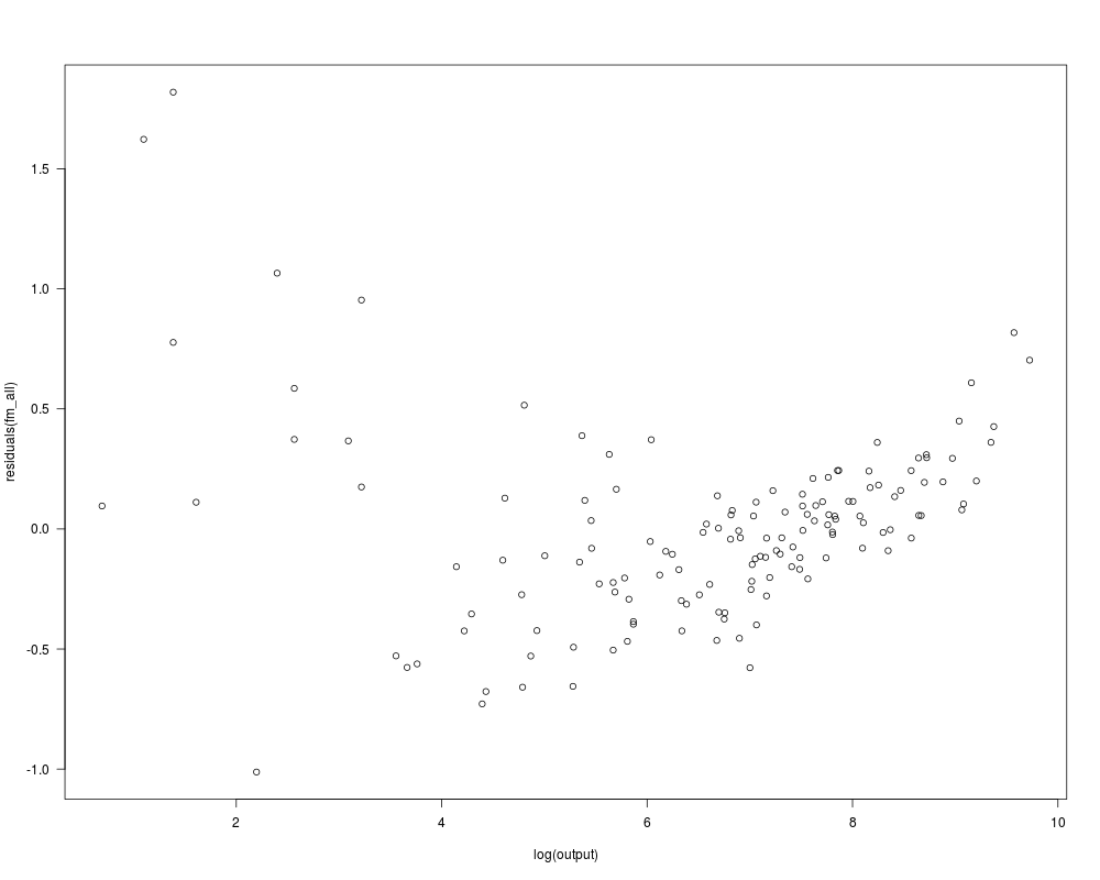
## Example 7.3
## Cobb-Douglas cost function
fm_all <- lm(log(cost/fuel) ~ log(output) + log(labor/fuel) + log(capital/fuel),
  data = Electricity)
summary(fm_all)

## hypothesis of constant returns to scale
linearHypothesis(fm_all, "log(output) = 1")

## Figure 7.4
plot(residuals(fm_all) ~ log(output), data = Electricity)
## scaling seems to be different in Greene (2003) with logQ > 10?

## grouped functions
Electricity$group <- with(Electricity, cut(log(output), quantile(log(output), 0:5/5),
  include.lowest = TRUE, labels = 1:5))
fm_group <- lm(
  log(cost/fuel) ~ group/(log(output) + log(labor/fuel) + log(capital/fuel)) - 1,
  data = Electricity)

## Table 7.3 (close, but not quite)
round(rbind(coef(fm_all)[-1], matrix(coef(fm_group), nrow = 5)[,-1]), digits = 3)

## Table 7.4
## log quadratic cost function
fm_all2 <- lm(
  log(cost/fuel) ~ log(output) + I(log(output)^2) + log(labor/fuel) + log(capital/fuel),
  data = Electricity)
summary(fm_all2)


##########################
## Technological change ##
##########################

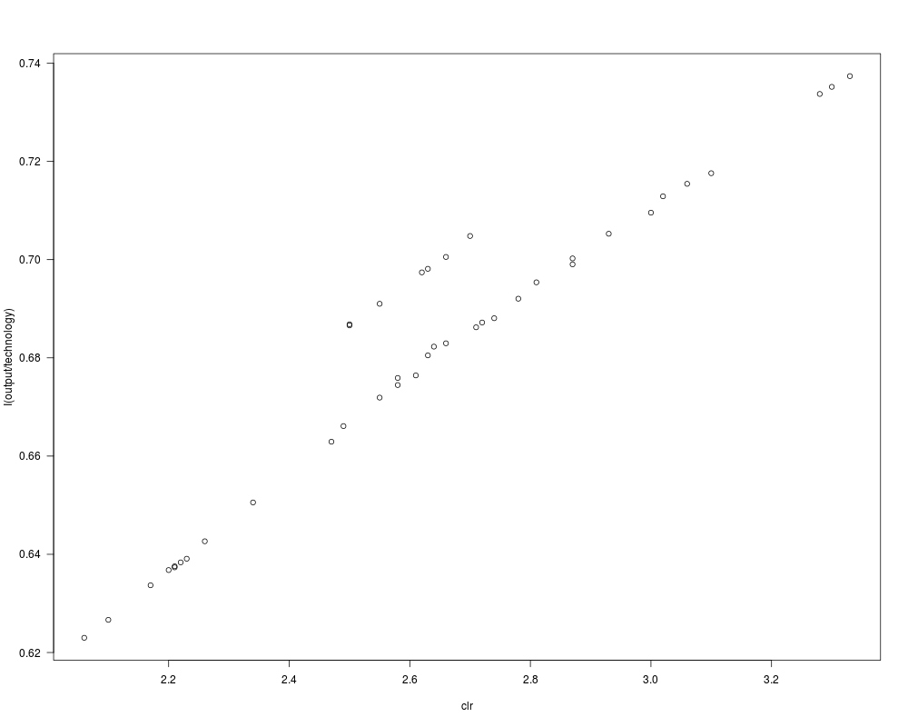
## Exercise 7.1
data("TechChange", package = "AER")
fm1 <- lm(I(output/technology) ~ log(clr), data = TechChange)
fm2 <- lm(I(output/technology) ~ I(1/clr), data = TechChange)
fm3 <- lm(log(output/technology) ~ log(clr), data = TechChange)
fm4 <- lm(log(output/technology) ~ I(1/clr), data = TechChange)

## Exercise 7.2 (a) and (c)
plot(I(output/technology) ~ clr, data = TechChange)
sctest(I(output/technology) ~ log(clr), data = TechChange,
  type = "Chow", point = c(1942, 1))


##################################
## Expenditure and default data ##
##################################

## full data set (F21.4)
data("CreditCard", package = "AER")

## extract data set F9.1
ccard <- CreditCard[1:100,]
ccard$income <- round(ccard$income, digits = 2)
ccard$expenditure <- round(ccard$expenditure, digits = 2)
ccard$age <- round(ccard$age + .01)
## suspicious:
CreditCard$age[CreditCard$age < 1]
## the first of these is also in TableF9.1 with 36 instead of 0.5:
ccard$age[79] <- 36

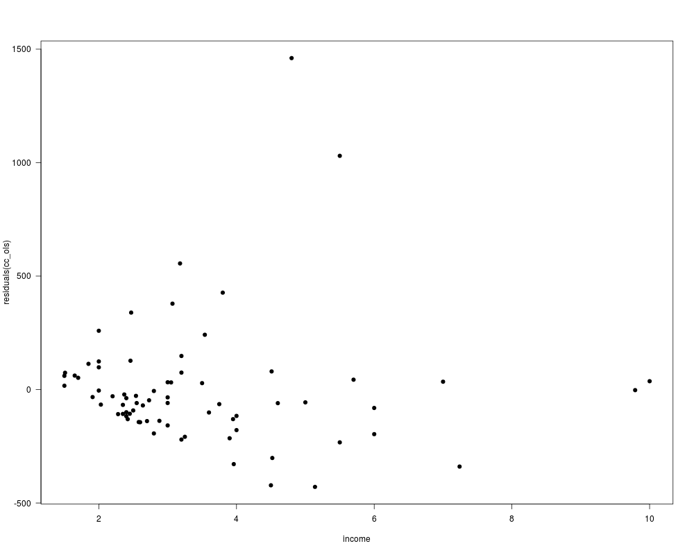
## Example 11.1
ccard <- ccard[order(ccard$income),]
ccard0 <- subset(ccard, expenditure > 0)
cc_ols <- lm(expenditure ~ age + owner + income + I(income^2), data = ccard0)

## Figure 11.1
plot(residuals(cc_ols) ~ income, data = ccard0, pch = 19)

## Table 11.1
mean(ccard$age)
prop.table(table(ccard$owner))
mean(ccard$income)

summary(cc_ols)
sqrt(diag(vcovHC(cc_ols, type = "HC0")))
sqrt(diag(vcovHC(cc_ols, type = "HC2"))) 
sqrt(diag(vcovHC(cc_ols, type = "HC1")))

bptest(cc_ols, ~ (age + income + I(income^2) + owner)^2 + I(age^2) + I(income^4),
  data = ccard0)
gqtest(cc_ols)
bptest(cc_ols, ~ income + I(income^2), data = ccard0, studentize = FALSE)
bptest(cc_ols, ~ income + I(income^2), data = ccard0)

## Table 11.2, WLS and FGLS
cc_wls1 <- lm(expenditure ~ age + owner + income + I(income^2), weights = 1/income,
  data = ccard0)
cc_wls2 <- lm(expenditure ~ age + owner + income + I(income^2), weights = 1/income^2,
  data = ccard0)

auxreg1 <- lm(log(residuals(cc_ols)^2) ~ log(income), data = ccard0)
cc_fgls1 <- lm(expenditure ~ age + owner + income + I(income^2),
  weights = 1/exp(fitted(auxreg1)), data = ccard0)

auxreg2 <- lm(log(residuals(cc_ols)^2) ~ income + I(income^2), data = ccard0)
cc_fgls2 <- lm(expenditure ~ age + owner + income + I(income^2),
  weights = 1/exp(fitted(auxreg2)), data = ccard0)

alphai <- coef(lm(log(residuals(cc_ols)^2) ~ log(income), data = ccard0))[2]
alpha <- 0
while(abs((alphai - alpha)/alpha) > 1e-7) {
  alpha <- alphai
  cc_fgls3 <- lm(expenditure ~ age + owner + income + I(income^2), weights = 1/income^alpha,
    data = ccard0)
  alphai <- coef(lm(log(residuals(cc_fgls3)^2) ~ log(income), data = ccard0))[2]
}
alpha ## 1.7623 for Greene
cc_fgls3 <- lm(expenditure ~ age + owner + income + I(income^2), weights = 1/income^alpha,
  data = ccard0)

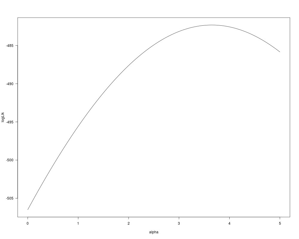
llik <- function(alpha)
  -logLik(lm(expenditure ~ age + owner + income + I(income^2), weights = 1/income^alpha,
    data = ccard0))
plot(0:100/20, -sapply(0:100/20, llik), type = "l", xlab = "alpha", ylab = "logLik")
alpha <- optimize(llik, interval = c(0, 5))$minimum
cc_fgls4 <- lm(expenditure ~ age + owner + income + I(income^2), weights = 1/income^alpha,
  data = ccard0)

## Table 11.2
cc_fit <- list(cc_ols, cc_wls1, cc_wls2, cc_fgls2, cc_fgls1, cc_fgls3, cc_fgls4)
t(sapply(cc_fit, coef))
t(sapply(cc_fit, function(obj) sqrt(diag(vcov(obj)))))

## Table 21.21, Poisson and logit models
cc_pois <- glm(reports ~ age + income + expenditure, data = CreditCard, family = poisson)
summary(cc_pois)
logLik(cc_pois)
xhat <- colMeans(CreditCard[, c("age", "income", "expenditure")])
xhat <- as.data.frame(t(xhat))
lambda <- predict(cc_pois, newdata = xhat, type = "response")
ppois(0, lambda) * nrow(CreditCard)

cc_logit <- glm(factor(reports > 0) ~ age + income + owner,
  data = CreditCard, family = binomial)
summary(cc_logit)
logLik(cc_logit)

## Table 21.21, "split population model"
library("pscl")
cc_zip <- zeroinfl(reports ~ age + income + expenditure | age + income + owner,
  data = CreditCard)
summary(cc_zip)
sum(predict(cc_zip, type = "prob")[,1])


###################################
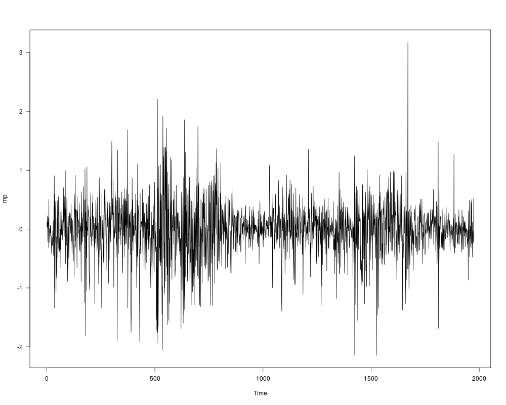
## DEM/GBP exchange rate returns ##
###################################

## data as given by Greene (2003)
data("MarkPound")
mp <- round(MarkPound, digits = 6)

## Figure 11.3 in Greene (2003)
plot(mp)

## Example 11.8 in Greene (2003), Table 11.5
library("tseries")
mp_garch <- garch(mp, grad = "numerical")
summary(mp_garch)
logLik(mp_garch)  
## Greene (2003) also includes a constant and uses different
## standard errors (presumably computed from Hessian), here
## OPG standard errors are used. garchFit() in "fGarch"
## implements the approach used by Greene (2003).

## compare Errata to Greene (2003)
library("dynlm")
res <- residuals(dynlm(mp ~ 1))^2
mp_ols <- dynlm(res ~ L(res, 1:10))
summary(mp_ols)
logLik(mp_ols)
summary(mp_ols)$r.squared * length(residuals(mp_ols))


################################
## Grunfeld's investment data ##
################################

## subset of data with mistakes
data("Grunfeld", package = "AER")
ggr <- subset(Grunfeld, firm %in% c("General Motors", "US Steel",
  "General Electric", "Chrysler", "Westinghouse"))
ggr[c(26, 38), 1] <- c(261.6, 645.2)
ggr[32, 3] <- 232.6

## Tab. 13.4
fm_pool <- lm(invest ~ value + capital, data = ggr)
summary(fm_pool)
logLik(fm_pool)
## White correction
sqrt(diag(vcovHC(fm_pool, type = "HC0")))

## heteroskedastic FGLS
auxreg1 <- lm(residuals(fm_pool)^2 ~ firm - 1, data = ggr)
fm_pfgls <- lm(invest ~ value + capital, data = ggr, weights = 1/fitted(auxreg1))
summary(fm_pfgls)

## ML, computed as iterated FGLS
sigmasi <- fitted(lm(residuals(fm_pfgls)^2 ~ firm - 1 , data = ggr))
sigmas <- 0
while(any(abs((sigmasi - sigmas)/sigmas) > 1e-7)) {
   sigmas <- sigmasi
   fm_pfgls_i <- lm(invest ~ value + capital, data = ggr, weights = 1/sigmas)
   sigmasi <- fitted(lm(residuals(fm_pfgls_i)^2 ~ firm - 1 , data = ggr))
   }
fm_pmlh <- lm(invest ~ value + capital, data = ggr, weights = 1/sigmas)
summary(fm_pmlh)
logLik(fm_pmlh)

## Tab. 13.5
auxreg2 <- lm(residuals(fm_pfgls)^2 ~ firm - 1, data = ggr)
auxreg3 <- lm(residuals(fm_pmlh)^2 ~ firm - 1, data = ggr)
rbind(
  "OLS" = coef(auxreg1),
  "Het. FGLS" = coef(auxreg2),
  "Het. ML" = coef(auxreg3))


## Chapter 14: explicitly treat as panel data
library("plm")
pggr <- plm.data(ggr, c("firm", "year"))

## Tab. 14.1
library("systemfit")
fm_sur <- systemfit(invest ~ value + capital, data = pggr, method = "SUR",
  methodResidCov = "noDfCor")
fm_psur <- systemfit(invest ~ value + capital, data = pggr, method = "SUR", pooled = TRUE, 
  methodResidCov = "noDfCor", residCovWeighted = TRUE)

## Tab 14.2
fm_ols <- systemfit(invest ~ value + capital, data = pggr, method = "OLS")
fm_pols <- systemfit(invest ~ value + capital, data = pggr, method = "OLS", pooled = TRUE)
## or "by hand"
fm_gm <- lm(invest ~ value + capital, data = ggr, subset = firm == "General Motors")
mean(residuals(fm_gm)^2)   ## Greene uses MLE
## etc.
fm_pool <- lm(invest ~ value + capital, data = ggr)

## Tab. 14.3 (and Tab 13.4, cross-section ML)
## (not run due to long computation time)
## Not run: 
fm_ml <- systemfit(invest ~ value + capital, data = pggr, method = "SUR",
  methodResidCov = "noDfCor", maxiter = 1000, tol = 1e-10)
fm_pml <- systemfit(invest ~ value + capital, data = pggr, method = "SUR", pooled = TRUE, 
  methodResidCov = "noDfCor", residCovWeighted = TRUE, maxiter = 1000, tol = 1e-10)

## End(Not run)

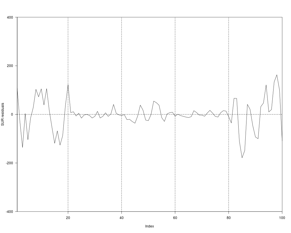
## Fig. 14.2
plot(unlist(residuals(fm_sur)[, c(3, 1, 2, 5, 4)]), 
  type = "l", ylab = "SUR residuals", ylim = c(-400, 400), xaxs = "i", yaxs = "i")
abline(v = c(20,40,60,80), h = 0, lty = 2)


###################
## Klein model I ##
###################

## data
data("KleinI", package = "AER")

## Tab. 15.3, OLS
library("dynlm")
fm_cons <- dynlm(consumption ~ cprofits + L(cprofits) + I(pwage + gwage), data = KleinI)
fm_inv <- dynlm(invest ~ cprofits + L(cprofits) + capital, data = KleinI)
fm_pwage <- dynlm(pwage ~ gnp + L(gnp) + I(time(gnp) - 1931), data = KleinI)
summary(fm_cons)
summary(fm_inv)
summary(fm_pwage)
## Notes:
##  - capital refers to previous year's capital stock -> no lag needed!
##  - trend used by Greene (p. 381, "time trend measured as years from 1931")
##    Maddala uses years since 1919

## preparation of data frame for systemfit
KI <- ts.intersect(KleinI, lag(KleinI, k = -1), dframe = TRUE)
names(KI) <- c(colnames(KleinI), paste("L", colnames(KleinI), sep = ""))
KI$trend <- (1921:1941) - 1931

library("systemfit")
system <- list(
  consumption = consumption ~ cprofits + Lcprofits + I(pwage + gwage),
  invest = invest ~ cprofits + Lcprofits + capital,
  pwage = pwage ~ gnp + Lgnp + trend)

## Tab. 15.3 OLS again
fm_ols <- systemfit(system, method = "OLS", data = KI)
summary(fm_ols)

## Tab. 15.3 2SLS, 3SLS, I3SLS
inst <- ~ Lcprofits + capital + Lgnp + gexpenditure + taxes + trend + gwage
fm_2sls <- systemfit(system, method = "2SLS", inst = inst,
  methodResidCov = "noDfCor", data = KI)

fm_3sls <- systemfit(system, method = "3SLS", inst = inst,
  methodResidCov = "noDfCor", data = KI)

fm_i3sls <- systemfit(system, method = "3SLS", inst = inst,
  methodResidCov = "noDfCor", maxiter = 100, data = KI)


############################################
## Transportation equipment manufacturing ##
############################################

## data
data("Equipment", package = "AER")

## Example 17.5
## Cobb-Douglas
fm_cd <- lm(log(valueadded/firms) ~ log(capital/firms) + log(labor/firms),
  data = Equipment)

## generalized Cobb-Douglas with Zellner-Revankar trafo
GCobbDouglas <- function(theta)
 lm(I(log(valueadded/firms) + theta * valueadded/firms) ~ log(capital/firms) + log(labor/firms),
     data = Equipment)

## yields classical Cobb-Douglas for theta = 0
fm_cd0 <- GCobbDouglas(0)

## ML estimation of generalized model
## choose starting values from classical model
par0 <- as.vector(c(coef(fm_cd0), 0, mean(residuals(fm_cd0)^2)))

## set up likelihood function
nlogL <- function(par) {
  beta <- par[1:3]
  theta <- par[4]
  sigma2 <- par[5]

  Y <- with(Equipment, valueadded/firms)
  K <- with(Equipment, capital/firms)
  L <- with(Equipment, labor/firms)

  rhs <- beta[1] + beta[2] * log(K) + beta[3] * log(L)
  lhs <- log(Y) + theta * Y

  rval <- sum(log(1 + theta * Y) - log(Y) +
    dnorm(lhs, mean = rhs, sd = sqrt(sigma2), log = TRUE))
  return(-rval)
}

## optimization
opt <- optim(par0, nlogL, hessian = TRUE)

## Table 17.2
opt$par
sqrt(diag(solve(opt$hessian)))[1:4]
-opt$value

## re-fit ML model
fm_ml <- GCobbDouglas(opt$par[4])
deviance(fm_ml)
sqrt(diag(vcov(fm_ml)))

## fit NLS model
rss <- function(theta) deviance(GCobbDouglas(theta))
optim(0, rss)
opt2 <- optimize(rss, c(-1, 1))
fm_nls <- GCobbDouglas(opt2$minimum)
-nlogL(c(coef(fm_nls), opt2$minimum, mean(residuals(fm_nls)^2)))


############################
## Municipal expenditures ##
############################

## Table 18.2
data("Municipalities", package = "AER")
summary(Municipalities)


###########################
## Program effectiveness ##
###########################

## Table 21.1, col. "Probit"
data("ProgramEffectiveness", package = "AER")
fm_probit <- glm(grade ~ average + testscore + participation,
  data = ProgramEffectiveness, family = binomial(link = "probit"))
summary(fm_probit)


####################################
## Labor force participation data ##
####################################

## data and transformations
data("PSID1976", package = "AER")
PSID1976$kids <- with(PSID1976, factor((youngkids + oldkids) > 0,
  levels = c(FALSE, TRUE), labels = c("no", "yes")))
PSID1976$nwincome <- with(PSID1976, (fincome - hours * wage)/1000)

## Example 4.1, Table 4.2
## (reproduced in Example 7.1, Table 7.1)
gr_lm <- lm(log(hours * wage) ~ age + I(age^2) + education + kids,
  data = PSID1976, subset = participation == "yes")
summary(gr_lm)
vcov(gr_lm)

## Example 4.5
summary(gr_lm)
## or equivalently
gr_lm1 <- lm(log(hours * wage) ~ 1, data = PSID1976, subset = participation == "yes")
anova(gr_lm1, gr_lm)

## Example 21.4, p. 681, and Tab. 21.3, p. 682
gr_probit1 <- glm(participation ~ age + I(age^2) + I(fincome/10000) + education + kids,
  data = PSID1976, family = binomial(link = "probit") )
gr_probit2 <- glm(participation ~ age + I(age^2) + I(fincome/10000) + education,
  data = PSID1976, family = binomial(link = "probit"))
gr_probit3 <- glm(participation ~ kids/(age + I(age^2) + I(fincome/10000) + education),
  data = PSID1976, family = binomial(link = "probit"))
## LR test of all coefficients
lrtest(gr_probit1)
## Chow-type test
lrtest(gr_probit2, gr_probit3)
## equivalently:
anova(gr_probit2, gr_probit3, test = "Chisq")
## Table 21.3
summary(gr_probit1)

## Example 22.8, Table 22.7, p. 786
library("sampleSelection")
gr_2step <- selection(participation ~ age + I(age^2) + fincome + education + kids, 
  wage ~ experience + I(experience^2) + education + city,
  data = PSID1976, method = "2step")
gr_ml <- selection(participation ~ age + I(age^2) + fincome + education + kids, 
  wage ~ experience + I(experience^2) + education + city,
  data = PSID1976, method = "ml")
gr_ols <- lm(wage ~ experience + I(experience^2) + education + city, 
  data = PSID1976, subset = participation == "yes")
## NOTE: ML estimates agree with Greene, 5e errata. 
## Standard errors are based on the Hessian (here), while Greene has BHHH/OPG.



####################
## Ship accidents ##
####################

## subset data
data("ShipAccidents", package = "AER")
sa <- subset(ShipAccidents, service > 0)

## Table 21.20
sa_full <- glm(incidents ~ type + construction + operation, family = poisson,
  data = sa, offset = log(service))
summary(sa_full)

sa_notype <- glm(incidents ~ construction + operation, family = poisson,
  data = sa, offset = log(service))
summary(sa_notype)

sa_noperiod <- glm(incidents ~ type + operation, family = poisson,
  data = sa, offset = log(service))
summary(sa_noperiod)

## model comparison
anova(sa_full, sa_notype, test = "Chisq")
anova(sa_full, sa_noperiod, test = "Chisq")

## test for overdispersion
dispersiontest(sa_full)
dispersiontest(sa_full, trafo = 2)


######################################
## Fair's extramarital affairs data ##
######################################

## data
data("Affairs", package = "AER")

## Tab. 22.3 and 22.4
fm_ols <- lm(affairs ~ age + yearsmarried + religiousness + occupation + rating,
  data = Affairs)
fm_probit <- glm(I(affairs > 0) ~ age + yearsmarried + religiousness + occupation + rating,
  data = Affairs, family = binomial(link = "probit"))

fm_tobit <- tobit(affairs ~ age + yearsmarried + religiousness + occupation + rating,
  data = Affairs)
fm_tobit2 <- tobit(affairs ~ age + yearsmarried + religiousness + occupation + rating,
  right = 4, data = Affairs)

fm_pois <- glm(affairs ~ age + yearsmarried + religiousness + occupation + rating,
  data = Affairs, family = poisson)

library("MASS")
fm_nb <- glm.nb(affairs ~ age + yearsmarried + religiousness + occupation + rating,
  data = Affairs)

## Tab. 22.6
library("pscl")
fm_zip <- zeroinfl(affairs ~ age + yearsmarried + religiousness + occupation + rating | age + 
  yearsmarried + religiousness + occupation + rating, data = Affairs)


######################
## Strike durations ##
######################

## data and package
data("StrikeDuration", package = "AER")
library("MASS")

## Table 22.10
fit_exp <- fitdistr(StrikeDuration$duration, "exponential")
fit_wei <- fitdistr(StrikeDuration$duration, "weibull")
fit_wei$estimate[2]^(-1)
fit_lnorm <- fitdistr(StrikeDuration$duration, "lognormal")
1/fit_lnorm$estimate[2]
exp(-fit_lnorm$estimate[1])
## Weibull and lognormal distribution have
## different parameterizations, see Greene p. 794

## Example 22.10
library("survival")
fm_wei <- survreg(Surv(duration) ~ uoutput, dist = "weibull", data = StrikeDuration)
summary(fm_wei)

Results

R version 3.3.1 (2016-06-21) -- "Bug in Your Hair"
Copyright (C) 2016 The R Foundation for Statistical Computing
Platform: x86_64-pc-linux-gnu (64-bit)

R is free software and comes with ABSOLUTELY NO WARRANTY.
You are welcome to redistribute it under certain conditions.
Type 'license()' or 'licence()' for distribution details.

R is a collaborative project with many contributors.
Type 'contributors()' for more information and
'citation()' on how to cite R or R packages in publications.

Type 'demo()' for some demos, 'help()' for on-line help, or
'help.start()' for an HTML browser interface to help.
Type 'q()' to quit R.

> library(AER)
Loading required package: car
Loading required package: lmtest
Loading required package: zoo

Attaching package: 'zoo'

The following objects are masked from 'package:base':

    as.Date, as.Date.numeric

Loading required package: sandwich
Loading required package: survival
> png(filename="/home/ddbj/snapshot/RGM3/R_CC/result/AER/Greene2003.Rd_%03d_medium.png", width=480, height=480)
> ### Name: Greene2003
> ### Title: Data and Examples from Greene (2003)
> ### Aliases: Greene2003
> ### Keywords: datasets
> 
> ### ** Examples
> 
> #####################################
> ## US consumption data (1970-1979) ##
> #####################################
> 
> ## Example 1.1
> data("USConsump1979", package = "AER")
> plot(expenditure ~ income, data = as.data.frame(USConsump1979), pch = 19)
> fm <- lm(expenditure ~ income, data = as.data.frame(USConsump1979))
> summary(fm)

Call:
lm(formula = expenditure ~ income, data = as.data.frame(USConsump1979))

Residuals:
    Min      1Q  Median      3Q     Max 
-11.291  -6.871   1.909   3.418  11.181 

Coefficients:
             Estimate Std. Error t value Pr(>|t|)    
(Intercept) -67.58065   27.91071  -2.421   0.0418 *  
income        0.97927    0.03161  30.983 1.28e-09 ***
---
Signif. codes:  0 '***' 0.001 '**' 0.01 '*' 0.05 '.' 0.1 ' ' 1

Residual standard error: 8.193 on 8 degrees of freedom
Multiple R-squared:  0.9917,	Adjusted R-squared:  0.9907 
F-statistic: 959.9 on 1 and 8 DF,  p-value: 1.28e-09

> abline(fm)
> 
> 
> #####################################
> ## US consumption data (1940-1950) ##
> #####################################
> 
> ## data
> data("USConsump1950", package = "AER")
> usc <- as.data.frame(USConsump1950)
> usc$war <- factor(usc$war, labels = c("no", "yes"))
> 
> ## Example 2.1
> plot(expenditure ~ income, data = usc, type = "n", xlim = c(225, 375), ylim = c(225, 350))
> with(usc, text(income, expenditure, time(USConsump1950)))
> 
> ## single model
> fm <- lm(expenditure ~ income, data = usc)
> summary(fm)

Call:
lm(formula = expenditure ~ income, data = usc)

Residuals:
    Min      1Q  Median      3Q     Max 
-35.347 -26.440   9.068  20.000  31.642 

Coefficients:
            Estimate Std. Error t value Pr(>|t|)  
(Intercept)  51.8951    80.8440   0.642   0.5369  
income        0.6848     0.2488   2.753   0.0224 *
---
Signif. codes:  0 '***' 0.001 '**' 0.01 '*' 0.05 '.' 0.1 ' ' 1

Residual standard error: 27.59 on 9 degrees of freedom
Multiple R-squared:  0.4571,	Adjusted R-squared:  0.3968 
F-statistic: 7.579 on 1 and 9 DF,  p-value: 0.02237

> 
> ## different intercepts for war yes/no
> fm2 <- lm(expenditure ~ income + war, data = usc)
> summary(fm2)

Call:
lm(formula = expenditure ~ income + war, data = usc)

Residuals:
    Min      1Q  Median      3Q     Max 
-14.598  -4.418  -2.352   7.242  11.101 

Coefficients:
             Estimate Std. Error t value Pr(>|t|)    
(Intercept)  14.49540   27.29948   0.531     0.61    
income        0.85751    0.08534  10.048 8.19e-06 ***
waryes      -50.68974    5.93237  -8.545 2.71e-05 ***
---
Signif. codes:  0 '***' 0.001 '**' 0.01 '*' 0.05 '.' 0.1 ' ' 1

Residual standard error: 9.195 on 8 degrees of freedom
Multiple R-squared:  0.9464,	Adjusted R-squared:  0.933 
F-statistic: 70.61 on 2 and 8 DF,  p-value: 8.26e-06

> 
> ## compare
> anova(fm, fm2)
Analysis of Variance Table

Model 1: expenditure ~ income
Model 2: expenditure ~ income + war
  Res.Df    RSS Df Sum of Sq     F   Pr(>F)    
1      9 6850.0                                
2      8  676.5  1    6173.5 73.01 2.71e-05 ***
---
Signif. codes:  0 '***' 0.001 '**' 0.01 '*' 0.05 '.' 0.1 ' ' 1
> 
> ## visualize
> abline(fm, lty = 3)                                   
> abline(coef(fm2)[1:2])                                
> abline(sum(coef(fm2)[c(1, 3)]), coef(fm2)[2], lty = 2)
> 
> ## Example 3.2
> summary(fm)$r.squared
[1] 0.4571345
> summary(lm(expenditure ~ income, data = usc, subset = war == "no"))$r.squared
[1] 0.9369742
> summary(fm2)$r.squared
[1] 0.9463904
> 
> 
> ########################
> ## US investment data ##
> ########################
> 
> data("USInvest", package = "AER")
> 
> ## Chapter 3 in Greene (2003)
> ## transform (and round) data to match Table 3.1
> us <- as.data.frame(USInvest)
> us$invest <- round(0.1 * us$invest/us$price, digits = 3)
> us$gnp <- round(0.1 * us$gnp/us$price, digits = 3)
> us$inflation <- c(4.4, round(100 * diff(us$price)/us$price[-15], digits = 2))
> us$trend <- 1:15
> us <- us[, c(2, 6, 1, 4, 5)]
> 
> ## p. 22-24
> coef(lm(invest ~ trend + gnp, data = us))
(Intercept)       trend         gnp 
-0.49459760 -0.01700063  0.64781939 
> coef(lm(invest ~ gnp, data = us))
(Intercept)         gnp 
-0.03333061  0.18388271 
> 
> ## Example 3.1, Table 3.2
> cor(us)[1,-1]
    trend       gnp  interest inflation 
0.7514213 0.8648613 0.5876756 0.4817416 
> pcor <- solve(cor(us))
> dcor <- 1/sqrt(diag(pcor))
> pcor <- (-pcor * (dcor %o% dcor))[1,-1]
> 
> ## Table 3.4
> fm  <- lm(invest ~ trend + gnp + interest + inflation, data = us)
> fm1 <- lm(invest ~ 1, data = us)
> anova(fm1, fm)
Analysis of Variance Table

Model 1: invest ~ 1
Model 2: invest ~ trend + gnp + interest + inflation
  Res.Df       RSS Df Sum of Sq      F    Pr(>F)    
1     14 0.0162736                                  
2     10 0.0004394  4  0.015834 90.089 8.417e-08 ***
---
Signif. codes:  0 '***' 0.001 '**' 0.01 '*' 0.05 '.' 0.1 ' ' 1
> 
> ## Example 4.1
> set.seed(123)
> w <- rnorm(10000)
> x <- rnorm(10000)
> eps <- 0.5 * w
> y <- 0.5 + 0.5 * x + eps
> b <- rep(0, 500)
> for(i in 1:500) {
+   ix <- sample(1:10000, 100)
+   b[i] <- lm.fit(cbind(1, x[ix]), y[ix])$coef[2]
+ }
> hist(b, breaks = 20, col = "lightgray")
> 
> 
> ###############################
> ## Longley's regression data ##
> ###############################
> 
> ## package and data
> data("Longley", package = "AER")
> library("dynlm")
> 
> ## Example 4.6
> fm1 <- dynlm(employment ~ time(employment) + price + gnp + armedforces,
+   data = Longley)
> fm2 <- update(fm1, end = 1961)
> cbind(coef(fm2), coef(fm1))
                          [,1]          [,2]
(Intercept)       1.459415e+06  1.169088e+06
time(employment) -7.217561e+02 -5.764643e+02
price            -1.811230e+02 -1.976807e+01
gnp               9.106778e-02  6.439397e-02
armedforces      -7.493705e-02 -1.014525e-02
> 
> ## Figure 4.3
> plot(rstandard(fm2), type = "b", ylim = c(-3, 3))
> abline(h = c(-2, 2), lty = 2)
> 
> 
> #########################################
> ## US gasoline market data (1960-1995) ##
> #########################################
> 
> ## data
> data("USGasG", package = "AER")
> 
> ## Greene (2003)
> ## Example 2.3
> fm <- lm(log(gas/population) ~ log(price) + log(income) + log(newcar) + log(usedcar),
+   data = as.data.frame(USGasG))
> summary(fm)

Call:
lm(formula = log(gas/population) ~ log(price) + log(income) + 
    log(newcar) + log(usedcar), data = as.data.frame(USGasG))

Residuals:
      Min        1Q    Median        3Q       Max 
-0.065042 -0.018842  0.001528  0.020786  0.058084 

Coefficients:
              Estimate Std. Error t value Pr(>|t|)    
(Intercept)  -12.34184    0.67489 -18.287   <2e-16 ***
log(price)    -0.05910    0.03248  -1.819   0.0786 .  
log(income)    1.37340    0.07563  18.160   <2e-16 ***
log(newcar)   -0.12680    0.12699  -0.998   0.3258    
log(usedcar)  -0.11871    0.08134  -1.459   0.1545    
---
Signif. codes:  0 '***' 0.001 '**' 0.01 '*' 0.05 '.' 0.1 ' ' 1

Residual standard error: 0.03304 on 31 degrees of freedom
Multiple R-squared:  0.958,	Adjusted R-squared:  0.9526 
F-statistic: 176.7 on 4 and 31 DF,  p-value: < 2.2e-16

> 
> ## Example 4.4
> ## estimates and standard errors (note different offset for intercept)
> coef(fm)
 (Intercept)   log(price)  log(income)  log(newcar) log(usedcar) 
-12.34184054  -0.05909513   1.37339912  -0.12679667  -0.11870847 
> sqrt(diag(vcov(fm)))
 (Intercept)   log(price)  log(income)  log(newcar) log(usedcar) 
  0.67489471   0.03248496   0.07562767   0.12699351   0.08133710 
> ## confidence interval
> confint(fm, parm = "log(income)")
               2.5 %   97.5 %
log(income) 1.219155 1.527643
> ## test linear hypothesis
> linearHypothesis(fm, "log(income) = 1")
Linear hypothesis test

Hypothesis:
log(income) = 1

Model 1: restricted model
Model 2: log(gas/population) ~ log(price) + log(income) + log(newcar) + 
    log(usedcar)

  Res.Df      RSS Df Sum of Sq      F   Pr(>F)    
1     32 0.060445                                 
2     31 0.033837  1  0.026608 24.377 2.57e-05 ***
---
Signif. codes:  0 '***' 0.001 '**' 0.01 '*' 0.05 '.' 0.1 ' ' 1
> 
> ## Figure 7.5
> plot(price ~ gas, data = as.data.frame(USGasG), pch = 19,
+   col = (time(USGasG) > 1973) + 1)
> legend("topleft", legend = c("after 1973", "up to 1973"), pch = 19, col = 2:1, bty = "n")
> 
> ## Example 7.6
> ## re-used in Example 8.3
> ## linear time trend
> ltrend <- 1:nrow(USGasG)
> ## shock factor
> shock <- factor(time(USGasG) > 1973, levels = c(FALSE, TRUE), labels = c("before", "after"))
> 
> ## 1960-1995
> fm1 <- lm(log(gas/population) ~ log(income) + log(price) + log(newcar) + log(usedcar) + ltrend,
+   data = as.data.frame(USGasG))
> summary(fm1)

Call:
lm(formula = log(gas/population) ~ log(income) + log(price) + 
    log(newcar) + log(usedcar) + ltrend, data = as.data.frame(USGasG))

Residuals:
      Min        1Q    Median        3Q       Max 
-0.055238 -0.017715  0.003659  0.016481  0.053522 

Coefficients:
               Estimate Std. Error t value Pr(>|t|)    
(Intercept)  -17.385790   1.679289 -10.353 2.03e-11 ***
log(income)    1.954626   0.192854  10.135 3.34e-11 ***
log(price)    -0.115530   0.033479  -3.451  0.00168 ** 
log(newcar)    0.205282   0.152019   1.350  0.18700    
log(usedcar)  -0.129274   0.071412  -1.810  0.08028 .  
ltrend        -0.019118   0.005957  -3.210  0.00316 ** 
---
Signif. codes:  0 '***' 0.001 '**' 0.01 '*' 0.05 '.' 0.1 ' ' 1

Residual standard error: 0.02898 on 30 degrees of freedom
Multiple R-squared:  0.9687,	Adjusted R-squared:  0.9635 
F-statistic: 185.8 on 5 and 30 DF,  p-value: < 2.2e-16

> ## pooled
> fm2 <- lm(
+   log(gas/population) ~ shock + log(income) + log(price) + log(newcar) + log(usedcar) + ltrend,
+   data = as.data.frame(USGasG))
> summary(fm2)

Call:
lm(formula = log(gas/population) ~ shock + log(income) + log(price) + 
    log(newcar) + log(usedcar) + ltrend, data = as.data.frame(USGasG))

Residuals:
      Min        1Q    Median        3Q       Max 
-0.045360 -0.019697  0.003931  0.015112  0.047550 

Coefficients:
               Estimate Std. Error t value Pr(>|t|)    
(Intercept)  -16.374402   1.456263 -11.244 4.33e-12 ***
shockafter     0.077311   0.021872   3.535  0.00139 ** 
log(income)    1.838167   0.167258  10.990 7.43e-12 ***
log(price)    -0.178005   0.033508  -5.312 1.06e-05 ***
log(newcar)    0.209842   0.129267   1.623  0.11534    
log(usedcar)  -0.128132   0.060721  -2.110  0.04359 *  
ltrend        -0.016862   0.005105  -3.303  0.00255 ** 
---
Signif. codes:  0 '***' 0.001 '**' 0.01 '*' 0.05 '.' 0.1 ' ' 1

Residual standard error: 0.02464 on 29 degrees of freedom
Multiple R-squared:  0.9781,	Adjusted R-squared:  0.9736 
F-statistic: 216.3 on 6 and 29 DF,  p-value: < 2.2e-16

> ## segmented
> fm3 <- lm(
+   log(gas/population) ~ shock/(log(income) + log(price) + log(newcar) + log(usedcar) + ltrend),
+   data = as.data.frame(USGasG))
> summary(fm3)

Call:
lm(formula = log(gas/population) ~ shock/(log(income) + log(price) + 
    log(newcar) + log(usedcar) + ltrend), data = as.data.frame(USGasG))

Residuals:
      Min        1Q    Median        3Q       Max 
-0.027349 -0.006332  0.001295  0.007159  0.022016 

Coefficients:
                         Estimate Std. Error t value Pr(>|t|)    
(Intercept)              -4.13439    5.03963  -0.820 0.420075    
shockafter               -4.74111    5.51576  -0.860 0.398538    
shockbefore:log(income)   0.42400    0.57973   0.731 0.471633    
shockafter:log(income)    1.01408    0.24904   4.072 0.000439 ***
shockbefore:log(price)    0.09455    0.24804   0.381 0.706427    
shockafter:log(price)    -0.24237    0.03490  -6.946  3.5e-07 ***
shockbefore:log(newcar)   0.58390    0.21670   2.695 0.012665 *  
shockafter:log(newcar)    0.33017    0.15789   2.091 0.047277 *  
shockbefore:log(usedcar) -0.33462    0.15215  -2.199 0.037738 *  
shockafter:log(usedcar)  -0.05537    0.04426  -1.251 0.222972    
shockbefore:ltrend        0.02637    0.01762   1.497 0.147533    
shockafter:ltrend        -0.01262    0.00329  -3.835 0.000798 ***
---
Signif. codes:  0 '***' 0.001 '**' 0.01 '*' 0.05 '.' 0.1 ' ' 1

Residual standard error: 0.01488 on 24 degrees of freedom
Multiple R-squared:  0.9934,	Adjusted R-squared:  0.9904 
F-statistic: 328.5 on 11 and 24 DF,  p-value: < 2.2e-16

> 
> ## Chow test
> anova(fm3, fm1)
Analysis of Variance Table

Model 1: log(gas/population) ~ shock/(log(income) + log(price) + log(newcar) + 
    log(usedcar) + ltrend)
Model 2: log(gas/population) ~ log(income) + log(price) + log(newcar) + 
    log(usedcar) + ltrend
  Res.Df       RSS Df Sum of Sq      F    Pr(>F)    
1     24 0.0053144                                  
2     30 0.0251878 -6 -0.019873 14.958 4.595e-07 ***
---
Signif. codes:  0 '***' 0.001 '**' 0.01 '*' 0.05 '.' 0.1 ' ' 1
> library("strucchange")
> sctest(log(gas/population) ~ log(income) + log(price) + log(newcar) + log(usedcar) + ltrend,
+   data = USGasG, point = c(1973, 1), type = "Chow")

	Chow test

data:  log(gas/population) ~ log(income) + log(price) + log(newcar) +     log(usedcar) + ltrend
F = 14.958, p-value = 4.595e-07

> ## Recursive CUSUM test
> rcus <- efp(log(gas/population) ~ log(income) + log(price) + log(newcar) + log(usedcar) + ltrend,
+    data = USGasG, type = "Rec-CUSUM")
> plot(rcus)
> sctest(rcus)

	Recursive CUSUM test

data:  rcus
S = 1.4977, p-value = 0.0002437

> ## Note: Greene's remark that the break is in 1984 (where the process crosses its boundary)
> ## is wrong. The break appears to be no later than 1976.
> 
> ## Example 12.2
> library("dynlm")
> resplot <- function(obj, bound = TRUE) {
+   res <- residuals(obj)
+   sigma <- summary(obj)$sigma
+   plot(res, ylab = "Residuals", xlab = "Year")
+   grid()
+   abline(h = 0)
+   if(bound) abline(h = c(-2, 2) * sigma, col = "red")  
+   lines(res)
+ }
> resplot(dynlm(log(gas/population) ~ log(price), data = USGasG))
> resplot(dynlm(log(gas/population) ~ log(price) + log(income), data = USGasG))
> resplot(dynlm(log(gas/population) ~ log(price) + log(income) + log(newcar) + log(usedcar) +
+   log(transport) + log(nondurable) + log(durable) +log(service) + ltrend, data = USGasG))
> ## different shock variable than in 7.6
> shock <- factor(time(USGasG) > 1974, levels = c(FALSE, TRUE), labels = c("before", "after"))
> resplot(dynlm(log(gas/population) ~ shock/(log(price) + log(income) + log(newcar) + log(usedcar) +
+   log(transport) + log(nondurable) + log(durable) + log(service) + ltrend), data = USGasG))
> ## NOTE: something seems to be wrong with the sigma estimates in the `full' models
> 
> ## Table 12.4, OLS
> fm <- dynlm(log(gas/population) ~ log(price) + log(income) + log(newcar) + log(usedcar),
+   data = USGasG)
> summary(fm)

Time series regression with "ts" data:
Start = 1960, End = 1995

Call:
dynlm(formula = log(gas/population) ~ log(price) + log(income) + 
    log(newcar) + log(usedcar), data = USGasG)

Residuals:
      Min        1Q    Median        3Q       Max 
-0.065042 -0.018842  0.001528  0.020786  0.058084 

Coefficients:
              Estimate Std. Error t value Pr(>|t|)    
(Intercept)  -12.34184    0.67489 -18.287   <2e-16 ***
log(price)    -0.05910    0.03248  -1.819   0.0786 .  
log(income)    1.37340    0.07563  18.160   <2e-16 ***
log(newcar)   -0.12680    0.12699  -0.998   0.3258    
log(usedcar)  -0.11871    0.08134  -1.459   0.1545    
---
Signif. codes:  0 '***' 0.001 '**' 0.01 '*' 0.05 '.' 0.1 ' ' 1

Residual standard error: 0.03304 on 31 degrees of freedom
Multiple R-squared:  0.958,	Adjusted R-squared:  0.9526 
F-statistic: 176.7 on 4 and 31 DF,  p-value: < 2.2e-16

> resplot(fm, bound = FALSE)
> dwtest(fm)

	Durbin-Watson test

data:  fm
DW = 0.6047, p-value = 3.387e-09
alternative hypothesis: true autocorrelation is greater than 0

> 
> ## ML
> g <- as.data.frame(USGasG)
> y <- log(g$gas/g$population)
> X <- as.matrix(cbind(log(g$price), log(g$income), log(g$newcar), log(g$usedcar)))
> arima(y, order = c(1, 0, 0), xreg = X)

Call:
arima(x = y, order = c(1, 0, 0), xreg = X)

Coefficients:
         ar1  intercept       X1      X2      X3       X4
      0.9304    -9.7548  -0.2082  1.0818  0.0884  -0.0350
s.e.  0.0554     1.1262   0.0337  0.1269  0.1186   0.0612

sigma^2 estimated as 0.0003094:  log likelihood = 93.37,  aic = -172.74
> 
> 
> #######################################
> ## US macroeconomic data (1950-2000) ##
> #######################################
> ## data and trend
> data("USMacroG", package = "AER")
> ltrend <- 0:(nrow(USMacroG) - 1)
> 
> ## Example 5.3
> ## OLS and IV regression
> library("dynlm")
> fm_ols <- dynlm(consumption ~ gdp, data = USMacroG)
> fm_iv <- dynlm(consumption ~ gdp | L(consumption) + L(gdp), data = USMacroG)
> 
> ## Hausman statistic
> library("MASS")
> b_diff <- coef(fm_iv) - coef(fm_ols)
> v_diff <- summary(fm_iv)$cov.unscaled - summary(fm_ols)$cov.unscaled
> (t(b_diff) %*% ginv(v_diff) %*% b_diff) / summary(fm_ols)$sigma^2
         [,1]
[1,] 9.703933
> 
> ## Wu statistic
> auxreg <- dynlm(gdp ~ L(consumption) + L(gdp), data = USMacroG)
> coeftest(dynlm(consumption ~ gdp + fitted(auxreg), data = USMacroG))[3,3] 
[1] 4.944502
> ## agrees with Greene (but not with errata)
> 
> ## Example 6.1
> ## Table 6.1
> fm6.1 <- dynlm(log(invest) ~ tbill + inflation + log(gdp) + ltrend, data = USMacroG)
> fm6.3 <- dynlm(log(invest) ~ I(tbill - inflation) + log(gdp) + ltrend, data = USMacroG)
> summary(fm6.1)

Time series regression with "ts" data:
Start = 1950(2), End = 2000(4)

Call:
dynlm(formula = log(invest) ~ tbill + inflation + log(gdp) + 
    ltrend, data = USMacroG)

Residuals:
     Min       1Q   Median       3Q      Max 
-0.22313 -0.05540 -0.00312  0.04246  0.31989 

Coefficients:
             Estimate Std. Error t value Pr(>|t|)    
(Intercept) -9.134091   1.366459  -6.684  2.3e-10 ***
tbill       -0.008598   0.003195  -2.691  0.00774 ** 
inflation    0.003306   0.002337   1.415  0.15872    
log(gdp)     1.930156   0.183272  10.532  < 2e-16 ***
ltrend      -0.005659   0.001488  -3.803  0.00019 ***
---
Signif. codes:  0 '***' 0.001 '**' 0.01 '*' 0.05 '.' 0.1 ' ' 1

Residual standard error: 0.08618 on 198 degrees of freedom
Multiple R-squared:  0.9798,	Adjusted R-squared:  0.9793 
F-statistic:  2395 on 4 and 198 DF,  p-value: < 2.2e-16

> summary(fm6.3)

Time series regression with "ts" data:
Start = 1950(2), End = 2000(4)

Call:
dynlm(formula = log(invest) ~ I(tbill - inflation) + log(gdp) + 
    ltrend, data = USMacroG)

Residuals:
      Min        1Q    Median        3Q       Max 
-0.227897 -0.054542 -0.002435  0.039993  0.313928 

Coefficients:
                      Estimate Std. Error t value Pr(>|t|)    
(Intercept)          -7.907158   1.200631  -6.586 3.94e-10 ***
I(tbill - inflation) -0.004427   0.002270  -1.950  0.05260 .  
log(gdp)              1.764062   0.160561  10.987  < 2e-16 ***
ltrend               -0.004403   0.001331  -3.308  0.00111 ** 
---
Signif. codes:  0 '***' 0.001 '**' 0.01 '*' 0.05 '.' 0.1 ' ' 1

Residual standard error: 0.0867 on 199 degrees of freedom
Multiple R-squared:  0.9794,	Adjusted R-squared:  0.9791 
F-statistic:  3154 on 3 and 199 DF,  p-value: < 2.2e-16

> deviance(fm6.1)
[1] 1.470565
> deviance(fm6.3)
[1] 1.495811
> vcov(fm6.1)[2,3] 
[1] -3.717454e-06
> 
> ## F test
> linearHypothesis(fm6.1, "tbill + inflation = 0")
Linear hypothesis test

Hypothesis:
tbill  + inflation = 0

Model 1: restricted model
Model 2: log(invest) ~ tbill + inflation + log(gdp) + ltrend

  Res.Df    RSS Df Sum of Sq      F  Pr(>F)  
1    199 1.4958                              
2    198 1.4706  1  0.025246 3.3991 0.06673 .
---
Signif. codes:  0 '***' 0.001 '**' 0.01 '*' 0.05 '.' 0.1 ' ' 1
> ## alternatively
> anova(fm6.1, fm6.3)
Analysis of Variance Table

Model 1: log(invest) ~ tbill + inflation + log(gdp) + ltrend
Model 2: log(invest) ~ I(tbill - inflation) + log(gdp) + ltrend
  Res.Df    RSS Df Sum of Sq      F  Pr(>F)  
1    198 1.4706                              
2    199 1.4958 -1 -0.025246 3.3991 0.06673 .
---
Signif. codes:  0 '***' 0.001 '**' 0.01 '*' 0.05 '.' 0.1 ' ' 1
> ## t statistic
> sqrt(anova(fm6.1, fm6.3)[2,5])
[1] 1.843672
>  
> ## Example 6.3
> ## Distributed lag model:
> ## log(Ct) = b0 + b1 * log(Yt) + b2 * log(C(t-1)) + u
> us <- log(USMacroG[, c(2, 5)])
> fm_distlag <- dynlm(log(consumption) ~ log(dpi) + L(log(consumption)),
+   data = USMacroG)
> summary(fm_distlag)

Time series regression with "ts" data:
Start = 1950(2), End = 2000(4)

Call:
dynlm(formula = log(consumption) ~ log(dpi) + L(log(consumption)), 
    data = USMacroG)

Residuals:
      Min        1Q    Median        3Q       Max 
-0.035243 -0.004606  0.000496  0.005147  0.041754 

Coefficients:
                    Estimate Std. Error t value Pr(>|t|)    
(Intercept)         0.003142   0.010553   0.298  0.76624    
log(dpi)            0.074958   0.028727   2.609  0.00976 ** 
L(log(consumption)) 0.924625   0.028594  32.337  < 2e-16 ***
---
Signif. codes:  0 '***' 0.001 '**' 0.01 '*' 0.05 '.' 0.1 ' ' 1

Residual standard error: 0.008742 on 200 degrees of freedom
Multiple R-squared:  0.9997,	Adjusted R-squared:  0.9997 
F-statistic: 3.476e+05 on 2 and 200 DF,  p-value: < 2.2e-16

> 
> ## estimate and test long-run MPC 
> coef(fm_distlag)[2]/(1-coef(fm_distlag)[3])
 log(dpi) 
0.9944606 
> linearHypothesis(fm_distlag, "log(dpi) + L(log(consumption)) = 1")
Linear hypothesis test

Hypothesis:
log(dpi)  + L(log(consumption)) = 1

Model 1: restricted model
Model 2: log(consumption) ~ log(dpi) + L(log(consumption))

  Res.Df      RSS Df  Sum of Sq      F Pr(>F)
1    201 0.015295                            
2    200 0.015286  1 9.1197e-06 0.1193 0.7301
> ## correct, see errata
>  
> ## Example 6.4
> ## predict investiment in 2001(1)
> predict(fm6.1, interval = "prediction",
+   newdata = data.frame(tbill = 4.48, inflation = 5.262, gdp = 9316.8, ltrend = 204))
       fit      lwr      upr
1 7.331178 7.158229 7.504126
> 
> ## Example 7.7
> ## no GMM available in "strucchange"
> ## using OLS instead yields
> fs <- Fstats(log(m1/cpi) ~ log(gdp) + tbill, data = USMacroG,
+   vcov = NeweyWest, from = c(1957, 3), to = c(1991, 3))
> plot(fs)
> ## which looks somewhat similar ...
>  
> ## Example 8.2
> ## Ct = b0 + b1*Yt + b2*Y(t-1) + v
> fm1 <- dynlm(consumption ~ dpi + L(dpi), data = USMacroG)
> ## Ct = a0 + a1*Yt + a2*C(t-1) + u
> fm2 <- dynlm(consumption ~ dpi + L(consumption), data = USMacroG)
> 
> ## Cox test in both directions:
> coxtest(fm1, fm2)
Cox test

Model 1: consumption ~ dpi + L(dpi)
Model 2: consumption ~ dpi + L(consumption)
                Estimate Std. Error     z value  Pr(>|z|)    
fitted(M1) ~ M2 -284.908    0.01862 -15304.2817 < 2.2e-16 ***
fitted(M2) ~ M1    1.491    0.42735      3.4894 0.0004842 ***
---
Signif. codes:  0 '***' 0.001 '**' 0.01 '*' 0.05 '.' 0.1 ' ' 1
> ## ... and do the same for jtest() and encomptest().
> ## Notice that in this particular case two of them are coincident.
> jtest(fm1, fm2)
J test

Model 1: consumption ~ dpi + L(dpi)
Model 2: consumption ~ dpi + L(consumption)
                Estimate Std. Error t value  Pr(>|t|)    
M1 + fitted(M2)   1.0145    0.01614 62.8605 < 2.2e-16 ***
M2 + fitted(M1) -10.6766    1.48542 -7.1876 1.299e-11 ***
---
Signif. codes:  0 '***' 0.001 '**' 0.01 '*' 0.05 '.' 0.1 ' ' 1
> encomptest(fm1, fm2)
Encompassing test

Model 1: consumption ~ dpi + L(dpi)
Model 2: consumption ~ dpi + L(consumption)
Model E: consumption ~ dpi + L(dpi) + L(consumption)
          Res.Df Df        F    Pr(>F)    
M1 vs. ME    199 -1 3951.448 < 2.2e-16 ***
M2 vs. ME    199 -1   51.661 1.299e-11 ***
---
Signif. codes:  0 '***' 0.001 '**' 0.01 '*' 0.05 '.' 0.1 ' ' 1
> ## encomptest could also be performed `by hand' via
> fmE <- dynlm(consumption ~ dpi + L(dpi) + L(consumption), data = USMacroG)
> waldtest(fm1, fmE, fm2)
Wald test

Model 1: consumption ~ dpi + L(dpi)
Model 2: consumption ~ dpi + L(dpi) + L(consumption)
Model 3: consumption ~ dpi + L(consumption)
  Res.Df Df        F    Pr(>F)    
1    200                          
2    199  1 3951.448 < 2.2e-16 ***
3    200 -1   51.661 1.299e-11 ***
---
Signif. codes:  0 '***' 0.001 '**' 0.01 '*' 0.05 '.' 0.1 ' ' 1
> 
> ## Table 9.1
> fm_ols <- lm(consumption ~ dpi, data = as.data.frame(USMacroG))
> fm_nls <- nls(consumption ~ alpha + beta * dpi^gamma,
+   start = list(alpha = coef(fm_ols)[1], beta = coef(fm_ols)[2], gamma = 1),
+   control = nls.control(maxiter = 100), data = as.data.frame(USMacroG))
> summary(fm_ols)

Call:
lm(formula = consumption ~ dpi, data = as.data.frame(USMacroG))

Residuals:
    Min      1Q  Median      3Q     Max 
-191.42  -56.08    1.38   49.53  324.14 

Coefficients:
              Estimate Std. Error t value Pr(>|t|)    
(Intercept) -80.354749  14.305852  -5.617 6.38e-08 ***
dpi           0.921686   0.003872 238.054  < 2e-16 ***
---
Signif. codes:  0 '***' 0.001 '**' 0.01 '*' 0.05 '.' 0.1 ' ' 1

Residual standard error: 87.21 on 202 degrees of freedom
Multiple R-squared:  0.9964,	Adjusted R-squared:  0.9964 
F-statistic: 5.667e+04 on 1 and 202 DF,  p-value: < 2.2e-16

> summary(fm_nls)

Formula: consumption ~ alpha + beta * dpi^gamma

Parameters:
       Estimate Std. Error t value Pr(>|t|)    
alpha 458.79851   22.50141  20.390   <2e-16 ***
beta    0.10085    0.01091   9.244   <2e-16 ***
gamma   1.24483    0.01205 103.263   <2e-16 ***
---
Signif. codes:  0 '***' 0.001 '**' 0.01 '*' 0.05 '.' 0.1 ' ' 1

Residual standard error: 50.09 on 201 degrees of freedom

Number of iterations to convergence: 64 
Achieved convergence tolerance: 1.695e-06

> deviance(fm_ols)
[1] 1536322
> deviance(fm_nls)
[1] 504403.2
> vcov(fm_nls)
            alpha          beta         gamma
alpha 506.3136444 -0.2345464437  0.2575688047
beta   -0.2345464  0.0001190377 -0.0001314916
gamma   0.2575688 -0.0001314916  0.0001453206
> 
> ## Example 9.7
> ## F test
> fm_nls2 <- nls(consumption ~ alpha + beta * dpi,
+   start = list(alpha = coef(fm_ols)[1], beta = coef(fm_ols)[2]),
+   control = nls.control(maxiter = 100), data = as.data.frame(USMacroG))
> anova(fm_nls, fm_nls2)
Analysis of Variance Table

Model 1: consumption ~ alpha + beta * dpi^gamma
Model 2: consumption ~ alpha + beta * dpi
  Res.Df Res.Sum Sq Df   Sum Sq F value    Pr(>F)    
1    201     504403                                  
2    202    1536322 -1 -1031919  411.21 < 2.2e-16 ***
---
Signif. codes:  0 '***' 0.001 '**' 0.01 '*' 0.05 '.' 0.1 ' ' 1
> ## Wald test
> linearHypothesis(fm_nls, "gamma = 1")
Linear hypothesis test

Hypothesis:
gamma = 1

Model 1: restricted model
Model 2: consumption ~ alpha + beta * dpi^gamma

  Res.Df Df  Chisq Pr(>Chisq)    
1    202                         
2    201  1 412.47  < 2.2e-16 ***
---
Signif. codes:  0 '***' 0.001 '**' 0.01 '*' 0.05 '.' 0.1 ' ' 1
> 
> ## Example 9.8, Table 9.2
> usm <- USMacroG[, c("m1", "tbill", "gdp")]
> fm_lin <- lm(m1 ~ tbill + gdp, data = usm)
> fm_log <- lm(m1 ~ tbill + gdp, data = log(usm))
> ## PE auxiliary regressions
> aux_lin <- lm(m1 ~ tbill + gdp + I(fitted(fm_log) - log(fitted(fm_lin))), data = usm)
> aux_log <- lm(m1 ~ tbill + gdp + I(fitted(fm_lin) - exp(fitted(fm_log))), data = log(usm))
> coeftest(aux_lin)[4,]
    Estimate   Std. Error      t value     Pr(>|t|) 
2.093544e+02 2.675803e+01 7.823985e+00 2.900156e-13 
> coeftest(aux_log)[4,]
     Estimate    Std. Error       t value      Pr(>|t|) 
-4.188803e-05  2.613270e-04 -1.602897e-01  8.728146e-01 
> ## matches results from errata
> ## With lmtest >= 0.9-24:
> ## petest(fm_lin, fm_log)
> 
> ## Example 12.1
> fm_m1 <- dynlm(log(m1) ~ log(gdp) + log(cpi), data = USMacroG)
> summary(fm_m1)

Time series regression with "ts" data:
Start = 1950(1), End = 2000(4)

Call:
dynlm(formula = log(m1) ~ log(gdp) + log(cpi), data = USMacroG)

Residuals:
      Min        1Q    Median        3Q       Max 
-0.230620 -0.026026  0.008483  0.036407  0.205929 

Coefficients:
            Estimate Std. Error t value Pr(>|t|)    
(Intercept) -1.63306    0.22857  -7.145 1.62e-11 ***
log(gdp)     0.28705    0.04738   6.058 6.68e-09 ***
log(cpi)     0.97181    0.03377  28.775  < 2e-16 ***
---
Signif. codes:  0 '***' 0.001 '**' 0.01 '*' 0.05 '.' 0.1 ' ' 1

Residual standard error: 0.08288 on 201 degrees of freedom
Multiple R-squared:  0.9895,	Adjusted R-squared:  0.9894 
F-statistic:  9489 on 2 and 201 DF,  p-value: < 2.2e-16

> 
> ## Figure 12.1
> par(las = 1)
> plot(0, 0, type = "n", axes = FALSE,
+      xlim = c(1950, 2002), ylim = c(-0.3, 0.225),
+      xaxs = "i", yaxs = "i",
+      xlab = "Quarter", ylab = "", main = "Least Squares Residuals")
> box()
> axis(1, at = c(1950, 1963, 1976, 1989, 2002))
> axis(2, seq(-0.3, 0.225, by = 0.075))
> grid(4, 7, col = grey(0.6))
> abline(0, 0)
> lines(residuals(fm_m1), lwd = 2)
> 
> ## Example 12.3
> fm_pc <- dynlm(d(inflation) ~ unemp, data = USMacroG)
> summary(fm_pc)

Time series regression with "ts" data:
Start = 1950(3), End = 2000(4)

Call:
dynlm(formula = d(inflation) ~ unemp,