Longley's Regression Data

Description

US macroeconomic time series, 1947–1962.

Usage

data("Longley")

Format

An annual multiple time series from 1947 to 1962 with 4 variables.

employment

Number of people employed (in 1000s).

price

GNP deflator.

gnp

Gross national product.

armedforces

Number of people in the armed forces.

Details

An extended version of this data set, formatted as a "data.frame" is available as longley in base R.

Source

Online complements to Greene (2003). Table F4.2.

http://pages.stern.nyu.edu/~wgreene/Text/tables/tablelist5.htm

References

Greene, W.H. (2003). Econometric Analysis, 5th edition. Upper Saddle River, NJ: Prentice Hall.

Longley, J.W. (1967). An Appraisal of Least-Squares Programs from the Point of View of the User. Journal of the American Statistical Association, 62, 819–841.

See Also

longley, Greene2003

Examples

data("Longley")
library("dynlm")

## Example 4.6 in Greene (2003)
fm1 <- dynlm(employment ~ time(employment) + price + gnp + armedforces,
  data = Longley)
fm2 <- update(fm1, end = 1961)
cbind(coef(fm2), coef(fm1))

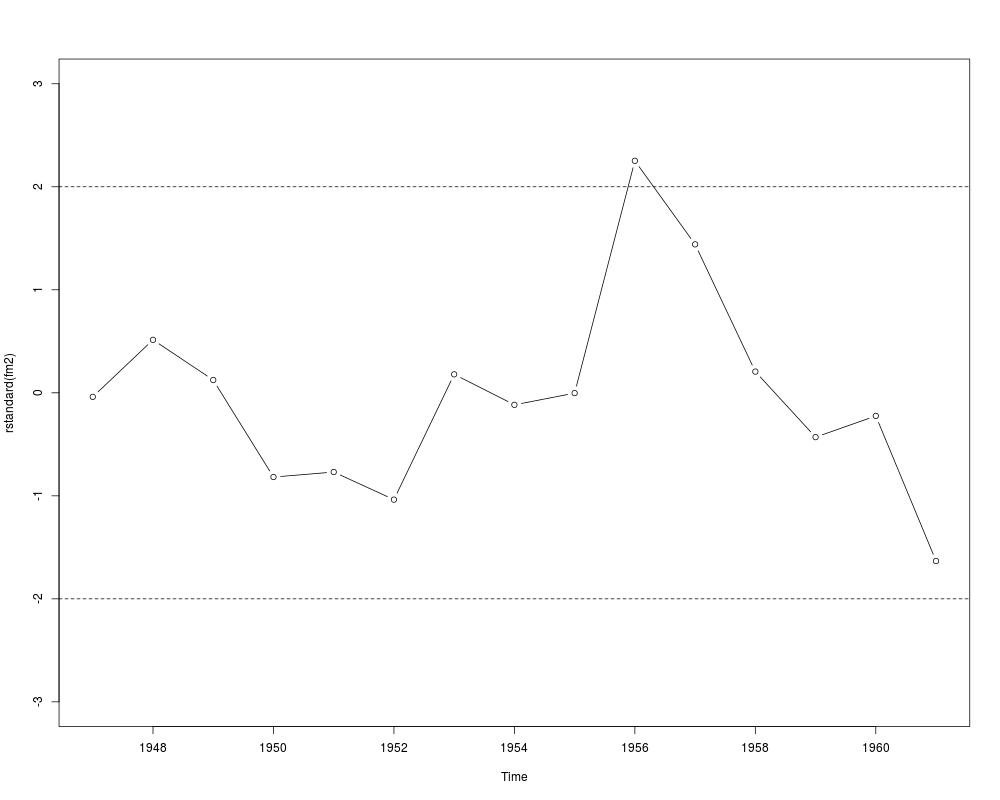
## Figure 4.3 in Greene (2003)
plot(rstandard(fm2), type = "b", ylim = c(-3, 3))
abline(h = c(-2, 2), lty = 2)

Results

R version 3.3.1 (2016-06-21) -- "Bug in Your Hair"
Copyright (C) 2016 The R Foundation for Statistical Computing
Platform: x86_64-pc-linux-gnu (64-bit)

R is free software and comes with ABSOLUTELY NO WARRANTY.
You are welcome to redistribute it under certain conditions.
Type 'license()' or 'licence()' for distribution details.

R is a collaborative project with many contributors.
Type 'contributors()' for more information and
'citation()' on how to cite R or R packages in publications.

Type 'demo()' for some demos, 'help()' for on-line help, or
'help.start()' for an HTML browser interface to help.
Type 'q()' to quit R.

> library(AER)
Loading required package: car
Loading required package: lmtest
Loading required package: zoo

Attaching package: 'zoo'

The following objects are masked from 'package:base':

    as.Date, as.Date.numeric

Loading required package: sandwich
Loading required package: survival
> png(filename="/home/ddbj/snapshot/RGM3/R_CC/result/AER/Longley.Rd_%03d_medium.png", width=480, height=480)
> ### Name: Longley
> ### Title: Longley's Regression Data
> ### Aliases: Longley
> ### Keywords: datasets
> 
> ### ** Examples
> 
> data("Longley")
> library("dynlm")
> 
> ## Example 4.6 in Greene (2003)
> fm1 <- dynlm(employment ~ time(employment) + price + gnp + armedforces,
+   data = Longley)
> fm2 <- update(fm1, end = 1961)
> cbind(coef(fm2), coef(fm1))
                          [,1]          [,2]
(Intercept)       1.459415e+06  1.169088e+06
time(employment) -7.217561e+02 -5.764643e+02
price            -1.811230e+02 -1.976807e+01
gnp               9.106778e-02  6.439397e-02
armedforces      -7.493705e-02 -1.014525e-02
> 
> ## Figure 4.3 in Greene (2003)
> plot(rstandard(fm2), type = "b", ylim = c(-3, 3))
> abline(h = c(-2, 2), lty = 2)
> 
> 
> 
> 
> 
> dev.off()
null device 
          1 
>