Supported by Dr. Osamu Ogasawara and  . . |
|
Last data update: 2014.03.03 |
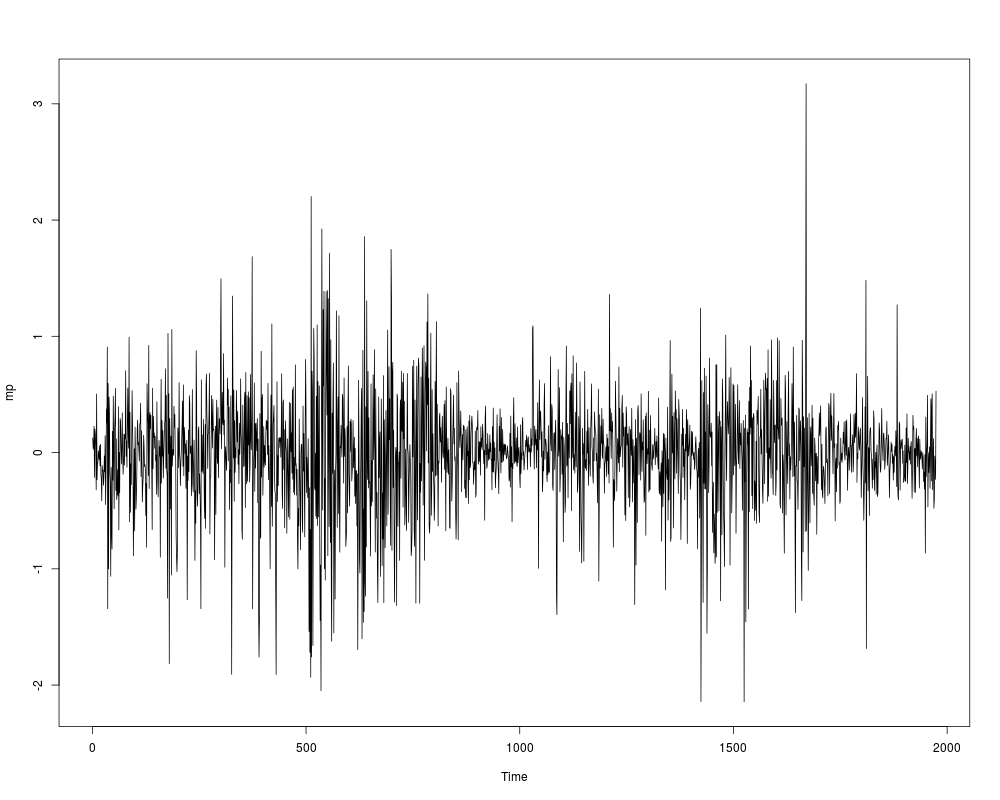
DEM/GBP Exchange Rate ReturnsDescriptionA daily time series of percentage returns of Deutsche mark/British pound (DEM/GBP) exchange rates from 1984-01-03 through 1991-12-31. Usagedata("MarkPound")
FormatA univariate time series of 1974 returns (exact dates unknown) for the DEM/GBP exchange rate. DetailsGreene (2003, Table F11.1) rounded the series to six digits while eight digits are given in
Bollerslev and Ghysels (1996). Here, we provide the original data. Using SourceJournal of Business & Economic Statistics Data Archive.
ReferencesBollerslev, T., and Ghysels, E. (1996). Periodic Autoregressive Conditional Heteroskedasticity. Journal of Business & Economic Statistics, 14, 139–151. Greene, W.H. (2003). Econometric Analysis, 5th edition. Upper Saddle River, NJ: Prentice Hall. See Also
Examples
## data as given by Greene (2003)
data("MarkPound")
mp <- round(MarkPound, digits = 6)

## Figure 11.3 in Greene (2003)
plot(mp)

## Example 11.8 in Greene (2003), Table 11.5
library("tseries")
mp_garch <- garch(mp, grad = "numerical")
summary(mp_garch)
logLik(mp_garch)
## Greene (2003) also includes a constant and uses different
## standard errors (presumably computed from Hessian), here
## OPG standard errors are used. garchFit() in "fGarch"
## implements the approach used by Greene (2003).

## compare Errata to Greene (2003)
library("dynlm")
res <- residuals(dynlm(mp ~ 1))^2
mp_ols <- dynlm(res ~ L(res, 1:10))
summary(mp_ols)
logLik(mp_ols)
summary(mp_ols)$r.squared * length(residuals(mp_ols))
Results
R version 3.3.1 (2016-06-21) -- "Bug in Your Hair"
Copyright (C) 2016 The R Foundation for Statistical Computing
Platform: x86_64-pc-linux-gnu (64-bit)

R is free software and comes with ABSOLUTELY NO WARRANTY.
You are welcome to redistribute it under certain conditions.
Type 'license()' or 'licence()' for distribution details.

R is a collaborative project with many contributors.
Type 'contributors()' for more information and
'citation()' on how to cite R or R packages in publications.

Type 'demo()' for some demos, 'help()' for on-line help, or
'help.start()' for an HTML browser interface to help.
Type 'q()' to quit R.

> library(AER)
Loading required package: car
Loading required package: lmtest
Loading required package: zoo

Attaching package: 'zoo'

The following objects are masked from 'package:base':

    as.Date, as.Date.numeric

Loading required package: sandwich
Loading required package: survival
> png(filename="/home/ddbj/snapshot/RGM3/R_CC/result/AER/MarkPound.Rd_%03d_medium.png", width=480, height=480)
> ### Name: MarkPound
> ### Title: DEM/GBP Exchange Rate Returns
> ### Aliases: MarkPound
> ### Keywords: datasets
>
> ### ** Examples
>
> ## data as given by Greene (2003)
> data("MarkPound")
> mp <- round(MarkPound, digits = 6)
>
> ## Figure 11.3 in Greene (2003)
> plot(mp)
>
> ## Example 11.8 in Greene (2003), Table 11.5
> library("tseries")
> mp_garch <- garch(mp, grad = "numerical")

 ***** ESTIMATION WITH NUMERICAL GRADIENT *****


     I     INITIAL X(I)        D(I)

     1     1.990169e-01     1.000e+00
     2     5.000000e-02     1.000e+00
     3     5.000000e-02     1.000e+00

    IT   NF      F         RELDF    PRELDF    RELDX   STPPAR   D*STEP   NPRELDF
     0    1 -5.449e+02
     1    3 -5.845e+02  6.78e-02  1.10e-01  2.5e-01  6.4e+03  1.0e-01  3.55e+02
     2    5 -5.913e+02  1.15e-02  3.08e-02  7.3e-02  4.6e+00  3.3e-02  4.87e+02
     3    6 -5.997e+02  1.40e-02  1.43e-02  7.8e-02  2.0e+00  3.3e-02  9.80e+01
     4    7 -6.126e+02  2.11e-02  2.71e-02  1.4e-01  2.0e+00  6.5e-02  6.24e+01
     5    8 -6.301e+02  2.77e-02  5.01e-02  1.8e-01  2.0e+00  1.3e-01  3.43e+01
     6    9 -6.537e+02  3.61e-02  4.89e-02  2.2e-01  2.0e+00  1.3e-01  1.19e+01
     7   11 -6.755e+02  3.24e-02  2.87e-02  1.6e-01  2.0e+00  1.3e-01  1.37e+01
     8   13 -6.878e+02  1.78e-02  1.71e-02  9.1e-02  2.0e+00  9.0e-02  2.84e+01
     9   16 -6.879e+02  2.73e-04  5.03e-04  1.4e-03  9.8e+00  1.8e-03  2.22e+01
    10   17 -6.881e+02  2.59e-04  2.67e-04  1.3e-03  2.1e+00  1.8e-03  1.82e+01
    11   18 -6.885e+02  6.02e-04  6.08e-04  2.9e-03  2.0e+00  3.6e-03  1.81e+01
    12   22 -6.963e+02  1.12e-02  1.21e-02  6.4e-02  2.0e+00  7.7e-02  1.73e+01
    13   26 -6.964e+02  1.07e-04  1.92e-04  5.9e-04  9.1e+00  8.2e-04  8.37e-01
    14   27 -6.965e+02  9.85e-05  1.00e-04  5.8e-04  2.4e+00  8.2e-04  6.52e-01
    15   28 -6.966e+02  1.80e-04  1.84e-04  1.1e-03  2.0e+00  1.6e-03  6.54e-01
    16   33 -7.031e+02  9.26e-03  1.18e-02  7.5e-02  1.9e+00  1.2e-01  6.40e-01
    17   35 -7.035e+02  5.47e-04  3.04e-03  1.3e-02  2.0e+00  1.9e-02  3.58e-01
    18   36 -7.039e+02  5.98e-04  4.77e-03  1.2e-02  2.0e+00  1.9e-02  1.55e-01
    19   37 -7.049e+02  1.45e-03  2.88e-03  1.2e-02  1.7e+00  1.9e-02  3.79e-03
    20   38 -7.054e+02  6.24e-04  2.27e-03  1.1e-02  1.7e+00  1.9e-02  1.82e-02
    21   39 -7.058e+02  5.68e-04  1.04e-03  1.1e-02  1.3e+00  1.9e-02  2.37e-03
    22   41 -7.064e+02  8.39e-04  9.73e-04  2.4e-02  3.0e-01  4.6e-02  1.01e-03
    23   42 -7.064e+02  1.86e-05  1.27e-04  4.7e-03  0.0e+00  8.1e-03  1.27e-04
    24   43 -7.064e+02  4.81e-05  4.69e-05  1.2e-03  0.0e+00  2.1e-03  4.69e-05
    25   44 -7.064e+02  4.68e-07  9.29e-07  7.7e-04  0.0e+00  1.5e-03  9.29e-07
    26   45 -7.064e+02  1.81e-07  2.01e-07  1.6e-04  0.0e+00  2.9e-04  2.01e-07
    27   46 -7.064e+02  5.17e-09  6.67e-09  4.1e-05  0.0e+00  9.0e-05  6.67e-09
    28   47 -7.064e+02  3.66e-10  3.68e-10  1.3e-05  0.0e+00  2.8e-05  3.68e-10
    29   48 -7.064e+02  1.98e-13  2.10e-13  1.6e-07  0.0e+00  3.1e-07  2.10e-13

 ***** RELATIVE FUNCTION CONVERGENCE *****

 FUNCTION    -7.064122e+02   RELDX        1.584e-07
 FUNC. EVALS      48         GRAD. EVALS     103
 PRELDF       2.102e-13      NPRELDF      2.102e-13

     I      FINAL X(I)        D(I)          G(I)

     1    1.086690e-02     1.000e+00     9.219e-04
     2    1.546040e-01     1.000e+00     4.441e-05
     3    8.044204e-01     1.000e+00     9.316e-05

> summary(mp_garch)

Call:
garch(x = mp, grad = "numerical")

Model:
GARCH(1,1)

Residuals:
      Min        1Q    Median        3Q       Max
-6.797392 -0.537032 -0.002637  0.552328  5.248670

Coefficient(s):
    Estimate  Std. Error  t value Pr(>|t|)
a0  0.010867    0.001297    8.376   <2e-16 ***
a1  0.154604    0.013882   11.137   <2e-16 ***
b1  0.804420    0.016046   50.133   <2e-16 ***
---
Signif. codes:  0 '***' 0.001 '**' 0.01 '*' 0.05 '.' 0.1 ' ' 1

Diagnostic Tests:
	Jarque Bera Test

data:  Residuals
X-squared = 1060, df = 2, p-value < 2.2e-16


	Box-Ljung test

data:  Squared.Residuals
X-squared = 2.4776, df = 1, p-value = 0.1155

> logLik(mp_garch)
'log Lik.' -1106.653 (df=3)
> ## Greene (2003) also includes a constant and uses different
> ## standard errors (presumably computed from Hessian), here
> ## OPG standard errors are used. garchFit() in "fGarch"
> ## implements the approach used by Greene (2003).
>
> ## compare Errata to Greene (2003)
> library("dynlm")
> res <- residuals(dynlm(mp ~ 1))^2
> mp_ols <- dynlm(res ~ L(res, 1:10))
> summary(mp_ols)

Time series regression with "ts" data:
Start = 11, End = 1974

Call:
dynlm(formula = res ~ L(res, 1:10))

Residuals:
    Min      1Q  Median      3Q     Max
-1.4937 -0.1560 -0.1042 -0.0065  9.7787

Coefficients:
                Estimate Std. Error t value Pr(>|t|)
(Intercept)     0.095733   0.014931   6.412 1.80e-10 ***
L(res, 1:10)1   0.161696   0.022595   7.156 1.17e-12 ***
L(res, 1:10)2   0.094938   0.022882   4.149 3.48e-05 ***
L(res, 1:10)3   0.051267   0.022973   2.232   0.0258 *
L(res, 1:10)4   0.034278   0.023003   1.490   0.1363
L(res, 1:10)5   0.121759   0.023015   5.290 1.36e-07 ***
L(res, 1:10)6  -0.007805   0.023015  -0.339   0.7346
L(res, 1:10)7   0.003673   0.023003   0.160   0.8731
L(res, 1:10)8   0.029509   0.022974   1.284   0.1991
L(res, 1:10)9   0.025063   0.022883   1.095   0.2735
L(res, 1:10)10  0.054212   0.022595   2.399   0.0165 *
---
Signif. codes:  0 '***' 0.001 '**' 0.01 '*' 0.05 '.' 0.1 ' ' 1

Residual standard error: 0.5005 on 1953 degrees of freedom
Multiple R-squared:  0.09795,	Adjusted R-squared:  0.09333
F-statistic: 21.21 on 10 and 1953 DF,  p-value: < 2.2e-16

> logLik(mp_ols)
'log Lik.' -1421.871 (df=12)
> summary(mp_ols)$r.squared * length(residuals(mp_ols))
[1] 192.3783
>
>
>
>
>
> dev.off()
null device
          1
>
|