Supported by Dr. Osamu Ogasawara and  . . |
|
Last data update: 2014.03.03 |
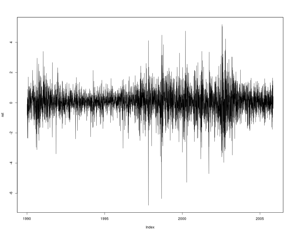
Daily NYSE Composite IndexDescriptionA daily time series from 1990 to 2005 of the New York Stock Exchange composite index. Usagedata("NYSESW")
FormatA daily univariate time series from 1990-01-02 to 2005-11-11 (of class
SourceOnline complements to Stock and Watson (2007). http://wps.aw.com/aw_stock_ie_2/ ReferencesStock, J.H. and Watson, M.W. (2007). Introduction to Econometrics, 2nd ed. Boston: Addison Wesley. See Also
Examples
## returns
data("NYSESW")
ret <- 100 * diff(log(NYSESW))
plot(ret)

## Stock and Watson (2007), p. 667, GARCH(1,1) model
library("tseries")
fm <- garch(coredata(ret))
summary(fm)
Results
R version 3.3.1 (2016-06-21) -- "Bug in Your Hair"
Copyright (C) 2016 The R Foundation for Statistical Computing
Platform: x86_64-pc-linux-gnu (64-bit)

R is free software and comes with ABSOLUTELY NO WARRANTY.
You are welcome to redistribute it under certain conditions.
Type 'license()' or 'licence()' for distribution details.

R is a collaborative project with many contributors.
Type 'contributors()' for more information and
'citation()' on how to cite R or R packages in publications.

Type 'demo()' for some demos, 'help()' for on-line help, or
'help.start()' for an HTML browser interface to help.
Type 'q()' to quit R.

> library(AER)
Loading required package: car
Loading required package: lmtest
Loading required package: zoo

Attaching package: 'zoo'

The following objects are masked from 'package:base':

    as.Date, as.Date.numeric

Loading required package: sandwich
Loading required package: survival
> png(filename="/home/ddbj/snapshot/RGM3/R_CC/result/AER/NYSESW.Rd_%03d_medium.png", width=480, height=480)
> ### Name: NYSESW
> ### Title: Daily NYSE Composite Index
> ### Aliases: NYSESW
> ### Keywords: datasets
>
> ### ** Examples
>
> ## returns
> data("NYSESW")
> ret <- 100 * diff(log(NYSESW))
> plot(ret)
>
> ## Stock and Watson (2007), p. 667, GARCH(1,1) model
> library("tseries")
> fm <- garch(coredata(ret))

 ***** ESTIMATION WITH ANALYTICAL GRADIENT *****


     I     INITIAL X(I)        D(I)

     1     7.247660e-01     1.000e+00
     2     5.000000e-02     1.000e+00
     3     5.000000e-02     1.000e+00

    IT   NF      F         RELDF    PRELDF    RELDX   STPPAR   D*STEP   NPRELDF
     0    1  1.503e+03
     1    3  1.487e+03  1.08e-02  2.29e-01  3.2e-01  1.7e+03  4.5e-01  1.96e+02
     2    4  1.481e+03  3.49e-03  6.05e-02  1.8e-01  2.7e+00  2.2e-01  6.80e+01
     3    5  1.406e+03  5.06e-02  6.85e-02  1.1e-01  2.3e+00  1.1e-01  8.55e+01
     4    7  1.374e+03  2.31e-02  2.63e-02  9.2e-02  1.2e+01  1.1e-01  6.91e+01
     5    9  1.356e+03  1.30e-02  2.07e-02  1.2e-01  4.0e+00  1.0e-01  1.06e+01
     6   10  1.330e+03  1.91e-02  2.08e-02  1.4e-01  2.0e+00  1.0e-01  1.47e+01
     7   11  1.297e+03  2.52e-02  3.20e-02  1.7e-01  2.0e+00  2.0e-01  1.11e+01
     8   13  1.290e+03  5.19e-03  1.02e-02  3.4e-02  2.9e+00  4.0e-02  1.85e+00
     9   14  1.278e+03  9.38e-03  1.03e-02  2.9e-02  2.0e+00  4.0e-02  2.39e+00
    10   15  1.261e+03  1.29e-02  1.58e-02  7.6e-02  2.0e+00  8.0e-02  1.92e+00
    11   16  1.227e+03  2.73e-02  3.26e-02  1.2e-01  2.0e+00  1.6e-01  2.11e+00
    12   18  1.223e+03  3.24e-03  9.12e-03  1.3e-02  1.8e+02  2.5e-02  4.47e+00
    13   19  1.212e+03  9.29e-03  9.02e-03  1.4e-02  2.0e+00  2.5e-02  1.59e+00
    14   22  1.168e+03  3.63e-02  3.40e-02  7.2e-02  1.8e+00  1.3e-01  1.70e+00
    15   24  1.162e+03  4.48e-03  7.20e-03  1.5e-02  2.0e+00  2.6e-02  5.64e+00
    16   25  1.150e+03  1.06e-02  1.12e-02  1.5e-02  2.0e+00  2.6e-02  3.37e+00
    17   27  1.135e+03  1.34e-02  1.43e-02  2.4e-02  2.0e+00  5.3e-02  3.34e+00
    18   28  1.118e+03  1.50e-02  3.01e-02  4.8e-02  1.9e+00  1.1e-01  9.31e-01
    19   31  1.111e+03  5.86e-03  8.61e-03  1.3e-03  4.0e+00  3.4e-03  9.54e-01
    20   33  1.102e+03  7.77e-03  1.33e-02  5.4e-03  1.6e+01  1.3e-02  1.18e+00
    21   37  1.102e+03  5.75e-04  9.10e-04  5.0e-04  3.8e+00  1.2e-03  3.59e-01
    22   39  1.101e+03  4.98e-04  5.37e-04  1.6e-03  2.1e+00  3.4e-03  2.75e-01
    23   40  1.100e+03  1.37e-03  1.55e-03  2.9e-03  2.0e+00  6.7e-03  2.23e-01
    24   43  1.096e+03  3.56e-03  6.62e-03  1.6e-02  1.8e+00  3.9e-02  9.44e-02
    25   45  1.095e+03  6.89e-04  8.79e-04  3.2e-03  1.0e+00  7.0e-03  1.17e-03
    26   47  1.095e+03  1.16e-04  1.90e-04  4.8e-04  1.0e+00  1.2e-03  3.08e-04
    27   48  1.095e+03  7.85e-07  9.55e-07  1.2e-04  0.0e+00  2.9e-04  9.55e-07
    28   49  1.095e+03  3.91e-08  9.27e-08  5.4e-05  0.0e+00  1.2e-04  9.27e-08
    29   50  1.095e+03  3.73e-09  1.07e-09  8.4e-06  0.0e+00  2.1e-05  1.07e-09
    30   51  1.095e+03 -1.54e-10  8.11e-11  1.6e-06  0.0e+00  4.0e-06  8.11e-11

 ***** RELATIVE FUNCTION CONVERGENCE *****

 FUNCTION     1.094921e+03   RELDX        1.590e-06
 FUNC. EVALS      51         GRAD. EVALS      30
 PRELDF       8.114e-11      NPRELDF      8.114e-11

     I      FINAL X(I)        D(I)          G(I)

     1    7.620546e-03     1.000e+00     3.522e-01
     2    7.019513e-02     1.000e+00     8.588e-02
     3    9.216098e-01     1.000e+00     1.571e-01

> summary(fm)

Call:
garch(x = coredata(ret))

Model:
GARCH(1,1)

Residuals:
     Min       1Q   Median       3Q      Max
-7.21895 -0.51459  0.06401  0.63914  4.31975

Coefficient(s):
    Estimate  Std. Error  t value Pr(>|t|)
a0  0.007621    0.001364    5.585 2.34e-08 ***
a1  0.070195    0.005063   13.863  < 2e-16 ***
b1  0.921610    0.005948  154.934  < 2e-16 ***
---
Signif. codes:  0 '***' 0.001 '**' 0.01 '*' 0.05 '.' 0.1 ' ' 1

Diagnostic Tests:
	Jarque Bera Test

data:  Residuals
X-squared = 805.62, df = 2, p-value < 2.2e-16


	Box-Ljung test

data:  Squared.Residuals
X-squared = 0.032173, df = 1, p-value = 0.8576

>
>
>
>
>
> dev.off()
null device
          1
>
|
Created & Maintained by Osamu Ogasawara (osamu.ogasawara@gmail.com) and 