PSID Earnings Data 1982

Description

Cross-section data originating from the Panel Study on Income Dynamics, 1982.

Usage

data("PSID1982")

Format

A data frame containing 595 observations on 12 variables.

experience

Years of full-time work experience.

weeks

Weeks worked.

occupation

factor. Is the individual a white-collar ("white") or blue-collar ("blue") worker?

industry

factor. Does the individual work in a manufacturing industry?

south

factor. Does the individual reside in the South?

smsa

factor. Does the individual reside in a SMSA (standard metropolitan statistical area)?

married

factor. Is the individual married?

gender

factor indicating gender.

union

factor. Is the individual's wage set by a union contract?

education

Years of education.

ethnicity

factor indicating ethnicity. Is the individual African-American ("afam") or not ("other")?

wage

Wage.

Details

PSID1982 is the cross-section for the year 1982 taken from a larger panel data set PSID7682 for the years 1976–1982, originating from Cornwell and Rupert (1988). Baltagi (2002) just uses the 1982 cross-section; hence PSID1982 is available as a standalone data set because it was included in AER prior to the availability of the full PSID7682 panel version.

Source

The data is from Baltagi (2002).

References

Baltagi, B.H. (2002). Econometrics, 3rd ed. Berlin, Springer.

Cornwell, C., and Rupert, P. (1988). Efficient Estimation with Panel Data: An Empirical Comparison of Instrumental Variables Estimators. Journal of Applied Econometrics, 3, 149–155.

See Also

PSID7682, Baltagi2002

Examples

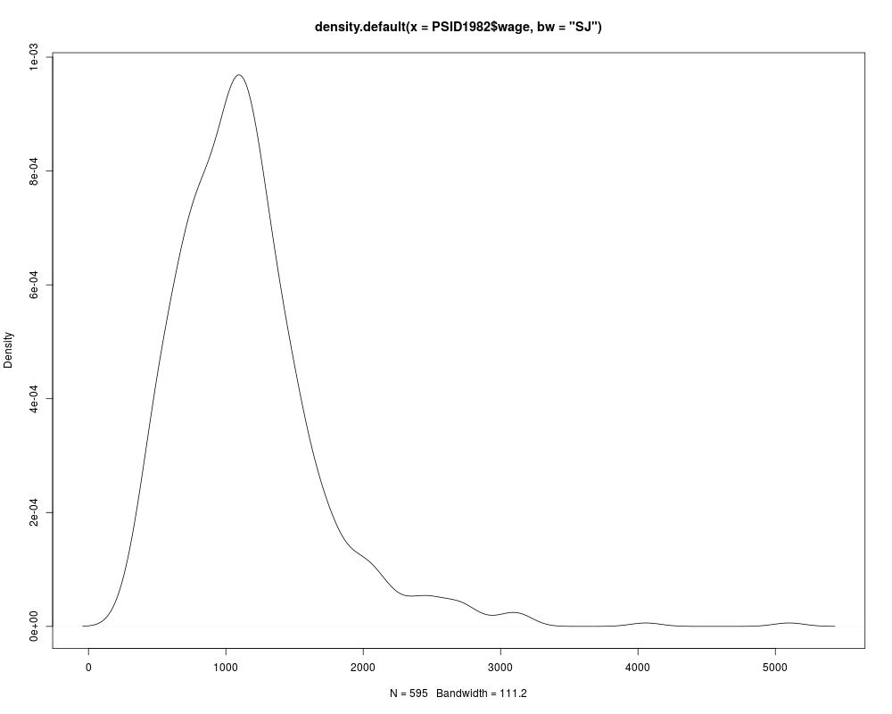
data("PSID1982")
plot(density(PSID1982$wage, bw = "SJ"))

## Baltagi (2002), Table 4.1
earn_lm <- lm(log(wage) ~ . + I(experience^2), data = PSID1982)
summary(earn_lm)

## Baltagi (2002), Table 13.1
union_lpm <- lm(I(as.numeric(union) - 1) ~ . - wage, data = PSID1982)
union_probit <- glm(union ~ . - wage, data = PSID1982, family = binomial(link = "probit"))
union_logit <- glm(union ~ . - wage, data = PSID1982, family = binomial)
## probit OK, logit and LPM rather different.

Results

R version 3.3.1 (2016-06-21) -- "Bug in Your Hair"
Copyright (C) 2016 The R Foundation for Statistical Computing
Platform: x86_64-pc-linux-gnu (64-bit)

R is free software and comes with ABSOLUTELY NO WARRANTY.
You are welcome to redistribute it under certain conditions.
Type 'license()' or 'licence()' for distribution details.

R is a collaborative project with many contributors.
Type 'contributors()' for more information and
'citation()' on how to cite R or R packages in publications.

Type 'demo()' for some demos, 'help()' for on-line help, or
'help.start()' for an HTML browser interface to help.
Type 'q()' to quit R.

> library(AER)
Loading required package: car
Loading required package: lmtest
Loading required package: zoo

Attaching package: 'zoo'

The following objects are masked from 'package:base':

    as.Date, as.Date.numeric

Loading required package: sandwich
Loading required package: survival
> png(filename="/home/ddbj/snapshot/RGM3/R_CC/result/AER/PSID1982.Rd_%03d_medium.png", width=480, height=480)
> ### Name: PSID1982
> ### Title: PSID Earnings Data 1982
> ### Aliases: PSID1982
> ### Keywords: datasets
> 
> ### ** Examples
> 
> data("PSID1982")
> plot(density(PSID1982$wage, bw = "SJ"))
> 
> ## Baltagi (2002), Table 4.1
> earn_lm <- lm(log(wage) ~ . + I(experience^2), data = PSID1982)
> summary(earn_lm)

Call:
lm(formula = log(wage) ~ . + I(experience^2), data = PSID1982)

Residuals:
    Min      1Q  Median      3Q     Max 
-1.0271 -0.2292  0.0155  0.2231  1.1314 

Coefficients:
                  Estimate Std. Error t value Pr(>|t|)    
(Intercept)      5.5900930  0.1901125  29.404  < 2e-16 ***
experience       0.0293801  0.0065241   4.503 8.09e-06 ***
weeks            0.0034128  0.0026776   1.275 0.202973    
occupationblue  -0.1615216  0.0369073  -4.376 1.43e-05 ***
industryyes      0.0846626  0.0291637   2.903 0.003836 ** 
southyes        -0.0587635  0.0309069  -1.901 0.057755 .  
smsayes          0.1661912  0.0295510   5.624 2.90e-08 ***
marriedyes       0.0952370  0.0489277   1.946 0.052077 .  
genderfemale    -0.3245574  0.0607294  -5.344 1.30e-07 ***
unionyes         0.1062775  0.0316755   3.355 0.000845 ***
education        0.0571935  0.0065910   8.678  < 2e-16 ***
ethnicityafam   -0.1904220  0.0544118  -3.500 0.000502 ***
I(experience^2) -0.0004860  0.0001268  -3.833 0.000141 ***
---
Signif. codes:  0 '***' 0.001 '**' 0.01 '*' 0.05 '.' 0.1 ' ' 1

Residual standard error: 0.3256 on 582 degrees of freedom
Multiple R-squared:  0.4597,	Adjusted R-squared:  0.4485 
F-statistic: 41.26 on 12 and 582 DF,  p-value: < 2.2e-16

> 
> ## Baltagi (2002), Table 13.1
> union_lpm <- lm(I(as.numeric(union) - 1) ~ . - wage, data = PSID1982)
> union_probit <- glm(union ~ . - wage, data = PSID1982, family = binomial(link = "probit"))
> union_logit <- glm(union ~ . - wage, data = PSID1982, family = binomial)
> ## probit OK, logit and LPM rather different.
> 
> 
> 
> 
> 
> dev.off()
null device 
          1 
>