Supported by Dr. Osamu Ogasawara and  . . |
|
Last data update: 2014.03.03 |
Data and Examples from Stock and Watson (2007)DescriptionThis manual page collects a list of examples from the book. Some solutions might not be exact and the list is certainly not complete. If you have suggestions for improvement (preferably in the form of code), please contact the package maintainer. ReferencesStock, J.H. and Watson, M.W. (2007). Introduction to Econometrics, 2nd ed. Boston: Addison Wesley. URL http://wps.aw.com/aw_stock_ie_2/0,12040,3332253-,00.html. See Also
Examples
###############################
## Current Population Survey ##
###############################
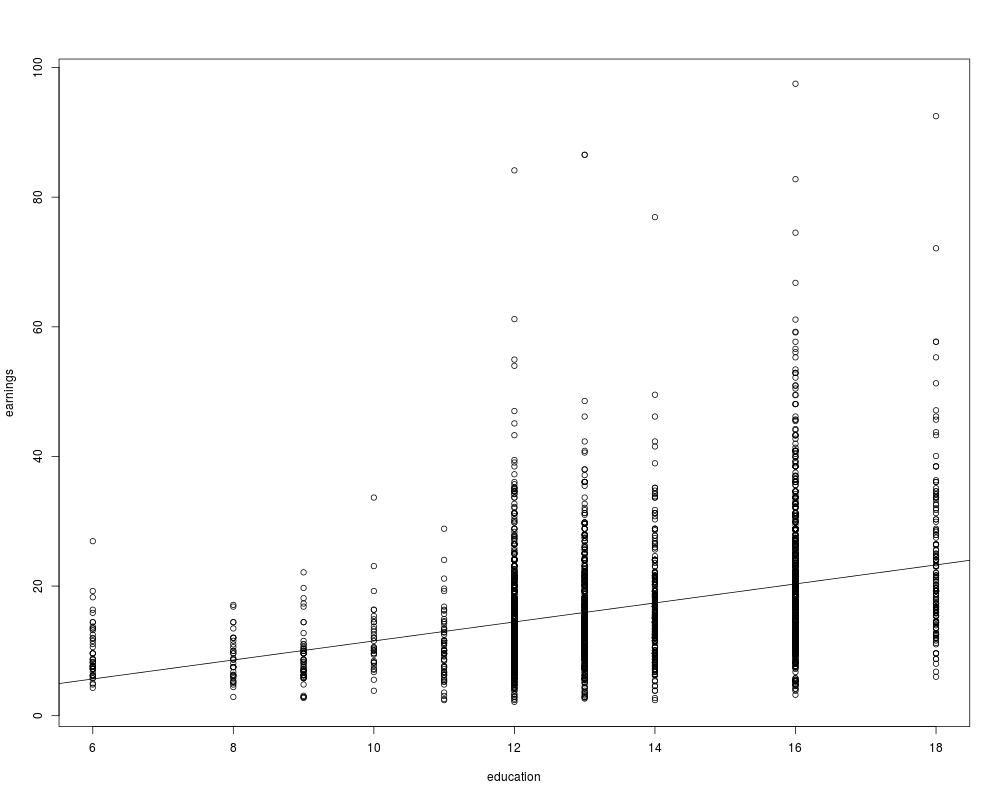
## p. 165
data("CPSSWEducation", package = "AER")
plot(earnings ~ education, data = CPSSWEducation)
fm <- lm(earnings ~ education, data = CPSSWEducation)
coeftest(fm, vcov = sandwich)
abline(fm)
############################
## California test scores ##
############################
## data and transformations
data("CASchools", package = "AER")
CASchools$stratio <- with(CASchools, students/teachers)
CASchools$score <- with(CASchools, (math + read)/2)
## p. 152
fm1 <- lm(score ~ stratio, data = CASchools)
coeftest(fm1, vcov = sandwich)
## p. 159
fm2 <- lm(score ~ I(stratio < 20), data = CASchools)
## p. 199
fm3 <- lm(score ~ stratio + english, data = CASchools)
## p. 224
fm4 <- lm(score ~ stratio + expenditure + english, data = CASchools)
## Table 7.1, p. 242 (numbers refer to columns)
fmc3 <- lm(score ~ stratio + english + lunch, data = CASchools)
fmc4 <- lm(score ~ stratio + english + calworks, data = CASchools)
fmc5 <- lm(score ~ stratio + english + lunch + calworks, data = CASchools)
## Equation 8.2, p. 258
fmquad <- lm(score ~ income + I(income^2), data = CASchools)
## Equation 8.11, p. 266
fmcub <- lm(score ~ income + I(income^2) + I(income^3), data = CASchools)
## Equation 8.23, p. 272
fmloglog <- lm(log(score) ~ log(income), data = CASchools)
## Equation 8.24, p. 274
fmloglin <- lm(log(score) ~ income, data = CASchools)
## Equation 8.26, p. 275
fmlinlogcub <- lm(score ~ log(income) + I(log(income)^2) + I(log(income)^3),
data = CASchools)
## Table 8.3, p. 292 (numbers refer to columns)
fmc2 <- lm(score ~ stratio + english + lunch + log(income), data = CASchools)
fmc7 <- lm(score ~ stratio + I(stratio^2) + I(stratio^3) + english + lunch + log(income),
data = CASchools)
#####################################
## Economics journal Subscriptions ##
#####################################
## data and transformed variables
data("Journals", package = "AER")
journals <- Journals[, c("subs", "price")]
journals$citeprice <- Journals$price/Journals$citations
journals$age <- 2000 - Journals$foundingyear
journals$chars <- Journals$charpp*Journals$pages/10^6
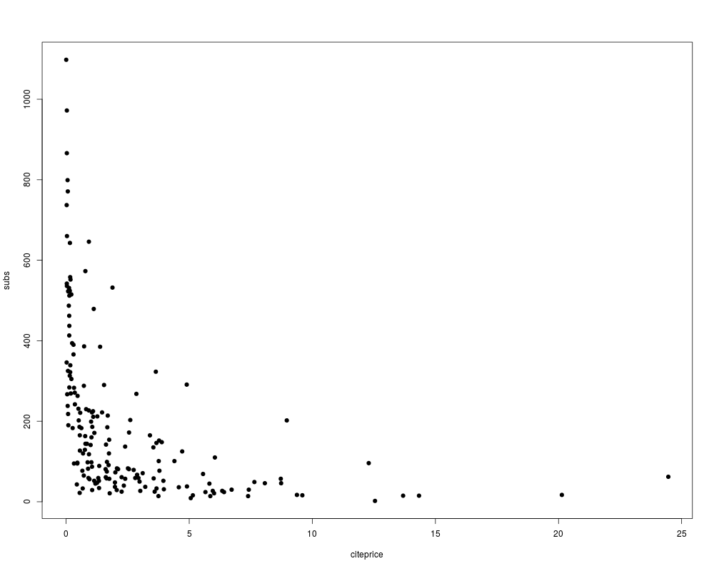
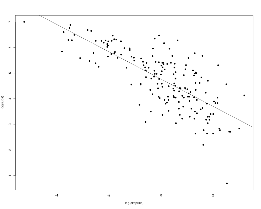
## Figure 8.9 (a) and (b)
plot(subs ~ citeprice, data = journals, pch = 19)
plot(log(subs) ~ log(citeprice), data = journals, pch = 19)
fm1 <- lm(log(subs) ~ log(citeprice), data = journals)
abline(fm1)
## Table 8.2, use HC1 for comparability with Stata
fm1 <- lm(subs ~ citeprice, data = log(journals))
fm2 <- lm(subs ~ citeprice + age + chars, data = log(journals))
fm3 <- lm(subs ~ citeprice + I(citeprice^2) + I(citeprice^3) +
age + I(age * citeprice) + chars, data = log(journals))
fm4 <- lm(subs ~ citeprice + age + I(age * citeprice) + chars, data = log(journals))
coeftest(fm1, vcov = vcovHC(fm1, type = "HC1"))
coeftest(fm2, vcov = vcovHC(fm2, type = "HC1"))
coeftest(fm3, vcov = vcovHC(fm3, type = "HC1"))
coeftest(fm4, vcov = vcovHC(fm4, type = "HC1"))
waldtest(fm3, fm4, vcov = vcovHC(fm3, type = "HC1"))
###############################
## Massachusetts test scores ##
###############################
## compare Massachusetts with California
data("MASchools", package = "AER")
data("CASchools", package = "AER")
CASchools$stratio <- with(CASchools, students/teachers)
CASchools$score4 <- with(CASchools, (math + read)/2)
## parts of Table 9.1, p. 330
vars <- c("score4", "stratio", "english", "lunch", "income")
cbind(
CA_mean = sapply(CASchools[, vars], mean),
CA_sd = sapply(CASchools[, vars], sd),
MA_mean = sapply(MASchools[, vars], mean),
MA_sd = sapply(MASchools[, vars], sd))
## Table 9.2, pp. 332--333, numbers refer to columns
MASchools$higheng <- with(MASchools, english > median(english))
fm1 <- lm(score4 ~ stratio, data = MASchools)
fm2 <- lm(score4 ~ stratio + english + lunch + log(income), data = MASchools)
fm3 <- lm(score4 ~ stratio + english + lunch + income + I(income^2) + I(income^3),
data = MASchools)
fm4 <- lm(score4 ~ stratio + I(stratio^2) + I(stratio^3) + english + lunch +
income + I(income^2) + I(income^3), data = MASchools)
fm5 <- lm(score4 ~ stratio + higheng + I(higheng * stratio) + lunch +
income + I(income^2) + I(income^3), data = MASchools)
fm6 <- lm(score4 ~ stratio + lunch + income + I(income^2) + I(income^3),
data = MASchools)
## for comparability with Stata use HC1 below
coeftest(fm1, vcov = vcovHC(fm1, type = "HC1"))
coeftest(fm2, vcov = vcovHC(fm2, type = "HC1"))
coeftest(fm3, vcov = vcovHC(fm3, type = "HC1"))
coeftest(fm4, vcov = vcovHC(fm4, type = "HC1"))
coeftest(fm5, vcov = vcovHC(fm5, type = "HC1"))
coeftest(fm6, vcov = vcovHC(fm6, type = "HC1"))
## Testing exclusion of groups of variables
fm3r <- update(fm3, . ~ . - I(income^2) - I(income^3))
waldtest(fm3, fm3r, vcov = vcovHC(fm3, type = "HC1"))
fm4r_str1 <- update(fm4, . ~ . - stratio - I(stratio^2) - I(stratio^3))
waldtest(fm4, fm4r_str1, vcov = vcovHC(fm4, type = "HC1"))
fm4r_str2 <- update(fm4, . ~ . - I(stratio^2) - I(stratio^3))
waldtest(fm4, fm4r_str2, vcov = vcovHC(fm4, type = "HC1"))
fm4r_inc <- update(fm4, . ~ . - I(income^2) - I(income^3))
waldtest(fm4, fm4r_inc, vcov = vcovHC(fm4, type = "HC1"))
fm5r_str <- update(fm5, . ~ . - stratio - I(higheng * stratio))
waldtest(fm5, fm5r_str, vcov = vcovHC(fm5, type = "HC1"))
fm5r_inc <- update(fm5, . ~ . - I(income^2) - I(income^3))
waldtest(fm5, fm5r_inc, vcov = vcovHC(fm5, type = "HC1"))
fm5r_high <- update(fm5, . ~ . - higheng - I(higheng * stratio))
waldtest(fm5, fm5r_high, vcov = vcovHC(fm5, type = "HC1"))
fm6r_inc <- update(fm6, . ~ . - I(income^2) - I(income^3))
waldtest(fm6, fm6r_inc, vcov = vcovHC(fm6, type = "HC1"))
##################################
## Home mortgage disclosure act ##
##################################
## data
data("HMDA", package = "AER")
## 11.1, 11.3, 11.7, 11.8 and 11.10, pp. 387--395
fm1 <- lm(I(as.numeric(deny) - 1) ~ pirat, data = HMDA)
fm2 <- lm(I(as.numeric(deny) - 1) ~ pirat + afam, data = HMDA)
fm3 <- glm(deny ~ pirat, family = binomial(link = "probit"), data = HMDA)
fm4 <- glm(deny ~ pirat + afam, family = binomial(link = "probit"), data = HMDA)
fm5 <- glm(deny ~ pirat + afam, family = binomial(link = "logit"), data = HMDA)
## Table 11.1, p. 401
mean(HMDA$pirat)
mean(HMDA$hirat)
mean(HMDA$lvrat)
mean(as.numeric(HMDA$chist))
mean(as.numeric(HMDA$mhist))
mean(as.numeric(HMDA$phist)-1)
prop.table(table(HMDA$insurance))
prop.table(table(HMDA$selfemp))
prop.table(table(HMDA$single))
prop.table(table(HMDA$hschool))
mean(HMDA$unemp)
prop.table(table(HMDA$condomin))
prop.table(table(HMDA$afam))
prop.table(table(HMDA$deny))
## Table 11.2, pp. 403--404, numbers refer to columns
HMDA$lvrat <- factor(ifelse(HMDA$lvrat < 0.8, "low",
ifelse(HMDA$lvrat >= 0.8 & HMDA$lvrat <= 0.95, "medium", "high")),
levels = c("low", "medium", "high"))
HMDA$mhist <- as.numeric(HMDA$mhist)
HMDA$chist <- as.numeric(HMDA$chist)
fm1 <- lm(I(as.numeric(deny) - 1) ~ afam + pirat + hirat + lvrat + chist + mhist +
phist + insurance + selfemp, data = HMDA)
fm2 <- glm(deny ~ afam + pirat + hirat + lvrat + chist + mhist + phist + insurance +
selfemp, family = binomial, data = HMDA)
fm3 <- glm(deny ~ afam + pirat + hirat + lvrat + chist + mhist + phist + insurance +
selfemp, family = binomial(link = "probit"), data = HMDA)
fm4 <- glm(deny ~ afam + pirat + hirat + lvrat + chist + mhist + phist + insurance +
selfemp + single + hschool + unemp, family = binomial(link = "probit"), data = HMDA)
fm5 <- glm(deny ~ afam + pirat + hirat + lvrat + chist + mhist + phist + insurance +
selfemp + single + hschool + unemp + condomin +
I(mhist==3) + I(mhist==4) + I(chist==3) + I(chist==4) + I(chist==5) + I(chist==6),
family = binomial(link = "probit"), data = HMDA)
fm6 <- glm(deny ~ afam * (pirat + hirat) + lvrat + chist + mhist + phist + insurance +
selfemp + single + hschool + unemp, family = binomial(link = "probit"), data = HMDA)
coeftest(fm1, vcov = sandwich)
fm4r <- update(fm4, . ~ . - single - hschool - unemp)
waldtest(fm4, fm4r, vcov = sandwich)
fm5r <- update(fm5, . ~ . - single - hschool - unemp)
waldtest(fm5, fm5r, vcov = sandwich)
fm6r <- update(fm6, . ~ . - single - hschool - unemp)
waldtest(fm6, fm6r, vcov = sandwich)
fm5r2 <- update(fm5, . ~ . - I(mhist==3) - I(mhist==4) - I(chist==3) - I(chist==4) -
I(chist==5) - I(chist==6))
waldtest(fm5, fm5r2, vcov = sandwich)
fm6r2 <- update(fm6, . ~ . - afam * (pirat + hirat) + pirat + hirat)
waldtest(fm6, fm6r2, vcov = sandwich)
fm6r3 <- update(fm6, . ~ . - afam * (pirat + hirat) + pirat + hirat + afam)
waldtest(fm6, fm6r3, vcov = sandwich)
#########################################################
## Shooting down the "More Guns Less Crime" hypothesis ##
#########################################################
## data
data("Guns", package = "AER")
## Empirical Exercise 10.1
fm1 <- lm(log(violent) ~ law, data = Guns)
fm2 <- lm(log(violent) ~ law + prisoners + density + income +
population + afam + cauc + male, data = Guns)
fm3 <- lm(log(violent) ~ law + prisoners + density + income +
population + afam + cauc + male + state, data = Guns)
fm4 <- lm(log(violent) ~ law + prisoners + density + income +
population + afam + cauc + male + state + year, data = Guns)
coeftest(fm1, vcov = sandwich)
coeftest(fm2, vcov = sandwich)
printCoefmat(coeftest(fm3, vcov = sandwich)[1:9,])
printCoefmat(coeftest(fm4, vcov = sandwich)[1:9,])
###########################
## US traffic fatalities ##
###########################
## data from Stock and Watson (2007)
data("Fatalities")
## add fatality rate (number of traffic deaths
## per 10,000 people living in that state in that year)
Fatalities$frate <- with(Fatalities, fatal/pop * 10000)
## add discretized version of minimum legal drinking age
Fatalities$drinkagec <- cut(Fatalities$drinkage,
breaks = 18:22, include.lowest = TRUE, right = FALSE)
Fatalities$drinkagec <- relevel(Fatalities$drinkagec, ref = 4)
## any punishment?
Fatalities$punish <- with(Fatalities,
factor(jail == "yes" | service == "yes", labels = c("no", "yes")))
## plm package
library("plm")
## for comparability with Stata we use HC1 below
## p. 351, Eq. (10.2)
f1982 <- subset(Fatalities, year == "1982")
fm_1982 <- lm(frate ~ beertax, data = f1982)
coeftest(fm_1982, vcov = vcovHC(fm_1982, type = "HC1"))
## p. 353, Eq. (10.3)
f1988 <- subset(Fatalities, year == "1988")
fm_1988 <- lm(frate ~ beertax, data = f1988)
coeftest(fm_1988, vcov = vcovHC(fm_1988, type = "HC1"))
## pp. 355, Eq. (10.8)
fm_diff <- lm(I(f1988$frate - f1982$frate) ~ I(f1988$beertax - f1982$beertax))
coeftest(fm_diff, vcov = vcovHC(fm_diff, type = "HC1"))
## pp. 360, Eq. (10.15)
## (1) via formula
fm_sfe <- lm(frate ~ beertax + state - 1, data = Fatalities)
## (2) by hand
fat <- with(Fatalities,
data.frame(frates = frate - ave(frate, state),
beertaxs = beertax - ave(beertax, state)))
fm_sfe2 <- lm(frates ~ beertaxs - 1, data = fat)
## (3) via plm()
fm_sfe3 <- plm(frate ~ beertax, data = Fatalities,
index = c("state", "year"), model = "within")
coeftest(fm_sfe, vcov = vcovHC(fm_sfe, type = "HC1"))[1,]
## uses different df in sd and p-value
coeftest(fm_sfe2, vcov = vcovHC(fm_sfe2, type = "HC1"))[1,]
## uses different df in p-value
coeftest(fm_sfe3, vcov = vcovHC(fm_sfe3, type = "HC1", method = "white1"))[1,]
## pp. 363, Eq. (10.21)
## via lm()
fm_stfe <- lm(frate ~ beertax + state + year - 1, data = Fatalities)
coeftest(fm_stfe, vcov = vcovHC(fm_stfe, type = "HC1"))[1,]
## via plm()
fm_stfe2 <- plm(frate ~ beertax, data = Fatalities,
index = c("state", "year"), model = "within", effect = "twoways")
coeftest(fm_stfe2, vcov = vcovHC) ## different
## p. 368, Table 10.1, numbers refer to cols.
fm1 <- plm(frate ~ beertax, data = Fatalities, index = c("state", "year"),
model = "pooling")
fm2 <- plm(frate ~ beertax, data = Fatalities, index = c("state", "year"),
model = "within")
fm3 <- plm(frate ~ beertax, data = Fatalities, index = c("state", "year"),
model = "within", effect = "twoways")
fm4 <- plm(frate ~ beertax + drinkagec + jail + service + miles + unemp + log(income),
data = Fatalities, index = c("state", "year"), model = "within", effect = "twoways")
fm5 <- plm(frate ~ beertax + drinkagec + jail + service + miles,
data = Fatalities, index = c("state", "year"), model = "within", effect = "twoways")
fm6 <- plm(frate ~ beertax + drinkage + punish + miles + unemp + log(income),
data = Fatalities, index = c("state", "year"), model = "within", effect = "twoways")
fm7 <- plm(frate ~ beertax + drinkagec + jail + service + miles + unemp + log(income),
data = Fatalities, index = c("state", "year"), model = "within", effect = "twoways")
## summaries not too close, s.e.s generally too small
coeftest(fm1, vcov = vcovHC)
coeftest(fm2, vcov = vcovHC)
coeftest(fm3, vcov = vcovHC)
coeftest(fm4, vcov = vcovHC)
coeftest(fm5, vcov = vcovHC)
coeftest(fm6, vcov = vcovHC)
coeftest(fm7, vcov = vcovHC)
######################################
## Cigarette consumption panel data ##
######################################
## data and transformations
data("CigarettesSW", package = "AER")
CigarettesSW$rprice <- with(CigarettesSW, price/cpi)
CigarettesSW$rincome <- with(CigarettesSW, income/population/cpi)
CigarettesSW$tdiff <- with(CigarettesSW, (taxs - tax)/cpi)
c1985 <- subset(CigarettesSW, year == "1985")
c1995 <- subset(CigarettesSW, year == "1995")
## convenience function: HC1 covariances
hc1 <- function(x) vcovHC(x, type = "HC1")
## Equations 12.9--12.11
fm_s1 <- lm(log(rprice) ~ tdiff, data = c1995)
coeftest(fm_s1, vcov = hc1)
fm_s2 <- lm(log(packs) ~ fitted(fm_s1), data = c1995)
fm_ivreg <- ivreg(log(packs) ~ log(rprice) | tdiff, data = c1995)
coeftest(fm_ivreg, vcov = hc1)
## Equation 12.15
fm_ivreg2 <- ivreg(log(packs) ~ log(rprice) + log(rincome) | log(rincome) + tdiff,
data = c1995)
coeftest(fm_ivreg2, vcov = hc1)
## Equation 12.16
fm_ivreg3 <- ivreg(log(packs) ~ log(rprice) + log(rincome) | log(rincome) + tdiff + I(tax/cpi),
data = c1995)
coeftest(fm_ivreg3, vcov = hc1)
## Table 12.1, p. 448
ydiff <- log(c1995$packs) - log(c1985$packs)
pricediff <- log(c1995$price/c1995$cpi) - log(c1985$price/c1985$cpi)
incdiff <- log(c1995$income/c1995$population/c1995$cpi) -
log(c1985$income/c1985$population/c1985$cpi)
taxsdiff <- (c1995$taxs - c1995$tax)/c1995$cpi - (c1985$taxs - c1985$tax)/c1985$cpi
taxdiff <- c1995$tax/c1995$cpi - c1985$tax/c1985$cpi
fm_diff1 <- ivreg(ydiff ~ pricediff + incdiff | incdiff + taxsdiff)
fm_diff2 <- ivreg(ydiff ~ pricediff + incdiff | incdiff + taxdiff)
fm_diff3 <- ivreg(ydiff ~ pricediff + incdiff | incdiff + taxsdiff + taxdiff)
coeftest(fm_diff1, vcov = hc1)
coeftest(fm_diff2, vcov = hc1)
coeftest(fm_diff3, vcov = hc1)
## checking instrument relevance
fm_rel1 <- lm(pricediff ~ taxsdiff + incdiff)
fm_rel2 <- lm(pricediff ~ taxdiff + incdiff)
fm_rel3 <- lm(pricediff ~ incdiff + taxsdiff + taxdiff)
linearHypothesis(fm_rel1, "taxsdiff = 0", vcov = hc1)
linearHypothesis(fm_rel2, "taxdiff = 0", vcov = hc1)
linearHypothesis(fm_rel3, c("taxsdiff = 0", "taxdiff = 0"), vcov = hc1)
## testing overidentifying restrictions (J test)
fm_or <- lm(residuals(fm_diff3) ~ incdiff + taxsdiff + taxdiff)
(fm_or_test <- linearHypothesis(fm_or, c("taxsdiff = 0", "taxdiff = 0"), test = "Chisq"))
## warning: df (and hence p-value) invalid above.
## correct df: # instruments - # endogenous variables
pchisq(fm_or_test[2,5], df.residual(fm_diff3) - df.residual(fm_or), lower.tail = FALSE)
#####################################################
## Project STAR: Student-teacher achievement ratio ##
#####################################################
## data
data("STAR", package = "AER")
## p. 488
fmk <- lm(I(readk + mathk) ~ stark, data = STAR)
fm1 <- lm(I(read1 + math1) ~ star1, data = STAR)
fm2 <- lm(I(read2 + math2) ~ star2, data = STAR)
fm3 <- lm(I(read3 + math3) ~ star3, data = STAR)
coeftest(fm3, vcov = sandwich)
## p. 489
fmke <- lm(I(readk + mathk) ~ stark + experiencek, data = STAR)
coeftest(fmke, vcov = sandwich)
## equivalently:
## - reshape data from wide into long format
## - fit a single model nested in grade
## (a) variables and their levels
nam <- c("star", "read", "math", "lunch", "school", "degree", "ladder",
"experience", "tethnicity", "system", "schoolid")
lev <- c("k", "1", "2", "3")
## (b) reshaping
star <- reshape(STAR, idvar = "id", ids = row.names(STAR),
times = lev, timevar = "grade", direction = "long",
varying = lapply(nam, function(x) paste(x, lev, sep = "")))
## (c) improve variable names and type
names(star)[5:15] <- nam
star$id <- factor(star$id)
star$grade <- factor(star$grade, levels = lev,
labels = c("kindergarten", "1st", "2nd", "3rd"))
rm(nam, lev)
## (d) model fitting
fm <- lm(I(read + math) ~ 0 + grade/star, data = star)
#################################################
## Quarterly US macroeconomic data (1957-2005) ##
#################################################
## data
data("USMacroSW", package = "AER")
library("dynlm")
usm <- ts.intersect(USMacroSW, 4 * 100 * diff(log(USMacroSW[, "cpi"])))
colnames(usm) <- c(colnames(USMacroSW), "infl")
## Equation 14.7, p. 536
fm_ar1 <- dynlm(d(infl) ~ L(d(infl)),
data = usm, start = c(1962,1), end = c(2004,4))
coeftest(fm_ar1, vcov = sandwich)
## Equation 14.13, p. 538
fm_ar4 <- dynlm(d(infl) ~ L(d(infl), 1:4),
data = usm, start = c(1962,1), end = c(2004,4))
coeftest(fm_ar4, vcov = sandwich)
## Equation 14.16, p. 542
fm_adl41 <- dynlm(d(infl) ~ L(d(infl), 1:4) + L(unemp),
data = usm, start = c(1962,1), end = c(2004,4))
coeftest(fm_adl41, vcov = sandwich)
## Equation 14.17, p. 542
fm_adl44 <- dynlm(d(infl) ~ L(d(infl), 1:4) + L(unemp, 1:4),
data = usm, start = c(1962,1), end = c(2004,4))
coeftest(fm_adl44, vcov = sandwich)
## Granger causality test mentioned on p. 547
waldtest(fm_ar4, fm_adl44, vcov = sandwich)
## Equation 14.28, p. 559
fm_sp1 <- dynlm(infl ~ log(gdpjp), start = c(1965,1), end = c(1981,4), data = usm)
coeftest(fm_sp1, vcov = sandwich)
## Equation 14.29, p. 559
fm_sp2 <- dynlm(infl ~ log(gdpjp), start = c(1982,1), end = c(2004,4), data = usm)
coeftest(fm_sp2, vcov = sandwich)
## Equation 14.34, p. 563: ADF by hand
fm_adf <- dynlm(d(infl) ~ L(infl) + L(d(infl), 1:4),
data = usm, start = c(1962,1), end = c(2004,4))
coeftest(fm_adf)
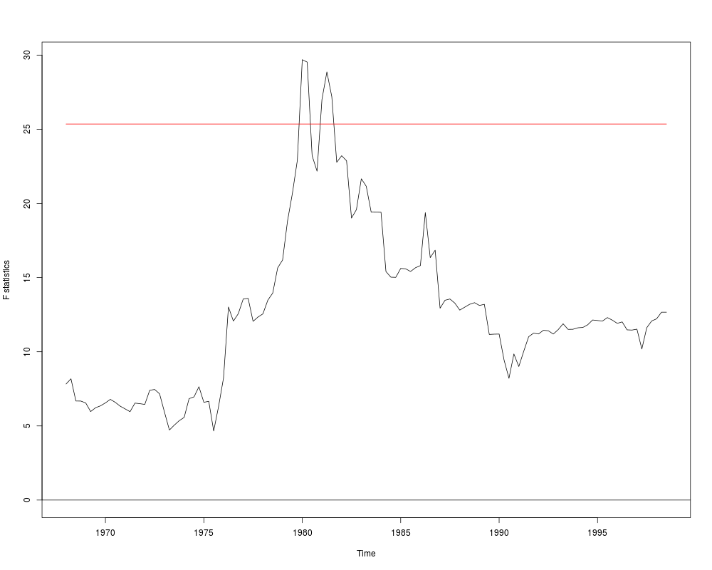
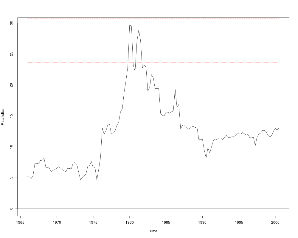
## Figure 14.5, p. 570
## SW perform partial break test of unemp coefs
## here full model is used
library("strucchange")
infl <- usm[, "infl"]
unemp <- usm[, "unemp"]
usm <- ts.intersect(diff(infl), lag(diff(infl), k = -1), lag(diff(infl), k = -2),
lag(diff(infl), k = -3), lag(diff(infl), k = -4), lag(unemp, k = -1),
lag(unemp, k = -2), lag(unemp, k = -3), lag(unemp, k = -4))
colnames(usm) <- c("dinfl", paste("dinfl", 1:4, sep = ""), paste("unemp", 1:4, sep = ""))
usm <- window(usm, start = c(1962, 1), end = c(2004, 4))
fs <- Fstats(dinfl ~ ., data = usm)
sctest(fs, type = "supF")
plot(fs)
## alternatively: re-use fm_adl44
mf <- model.frame(fm_adl44)
mf <- ts(as.matrix(mf), start = c(1962, 1), freq = 4)
colnames(mf) <- c("y", paste("x", 1:8, sep = ""))
ff <- as.formula(paste("y", "~", paste("x", 1:8, sep = "", collapse = " + ")))
fs <- Fstats(ff, data = mf, from = 0.1)
plot(fs)
lines(boundary(fs, alpha = 0.01), lty = 2, col = 2)
lines(boundary(fs, alpha = 0.1), lty = 3, col = 2)
##########################################
## Monthly US stock returns (1931-2002) ##
##########################################
## package and data
library("dynlm")
data("USStocksSW", package = "AER")
## Table 14.3, p. 540
fm1 <- dynlm(returns ~ L(returns), data = USStocksSW, start = c(1960,1))
coeftest(fm1, vcov = sandwich)
fm2 <- dynlm(returns ~ L(returns, 1:2), data = USStocksSW, start = c(1960,1))
waldtest(fm2, vcov = sandwich)
fm3 <- dynlm(returns ~ L(returns, 1:4), data = USStocksSW, start = c(1960,1))
waldtest(fm3, vcov = sandwich)
## Table 14.7, p. 574
fm4 <- dynlm(returns ~ L(returns) + L(d(dividend)),
data = USStocksSW, start = c(1960, 1))
fm5 <- dynlm(returns ~ L(returns, 1:2) + L(d(dividend), 1:2),
data = USStocksSW, start = c(1960, 1))
fm6 <- dynlm(returns ~ L(returns) + L(dividend),
data = USStocksSW, start = c(1960, 1))
##################################
## Price of frozen orange juice ##
##################################
## load data
data("FrozenJuice")
## Stock and Watson, p. 594
library("dynlm")
fm_dyn <- dynlm(d(100 * log(price/ppi)) ~ fdd, data = FrozenJuice)
coeftest(fm_dyn, vcov = vcovHC(fm_dyn, type = "HC1"))
## equivalently, returns can be computed 'by hand'
## (reducing the complexity of the formula notation)
fj <- ts.union(fdd = FrozenJuice[, "fdd"],
ret = 100 * diff(log(FrozenJuice[,"price"]/FrozenJuice[,"ppi"])))
fm_dyn <- dynlm(ret ~ fdd, data = fj)
## Stock and Watson, p. 595
fm_dl <- dynlm(ret ~ L(fdd, 0:6), data = fj)
coeftest(fm_dl, vcov = vcovHC(fm_dl, type = "HC1"))
## Stock and Watson, Table 15.1, p. 620, numbers refer to columns
## (1) Dynamic Multipliers
fm1 <- dynlm(ret ~ L(fdd, 0:18), data = fj)
coeftest(fm1, vcov = NeweyWest(fm1, lag = 7, prewhite = FALSE))
## (2) Cumulative Multipliers
fm2 <- dynlm(ret ~ L(d(fdd), 0:17) + L(fdd, 18), data = fj)
coeftest(fm2, vcov = NeweyWest(fm2, lag = 7, prewhite = FALSE))
## (3) Cumulative Multipliers, more lags in NW
coeftest(fm2, vcov = NeweyWest(fm2, lag = 14, prewhite = FALSE))
## (4) Cumulative Multipliers with monthly indicators
fm4 <- dynlm(ret ~ L(d(fdd), 0:17) + L(fdd, 18) + season(fdd), data = fj)
coeftest(fm4, vcov = NeweyWest(fm4, lag = 7, prewhite = FALSE))
## monthly indicators needed?
fm4r <- update(fm4, . ~ . - season(fdd))
waldtest(fm4, fm4r, vcov= NeweyWest(fm4, lag = 7, prewhite = FALSE)) ## close ...
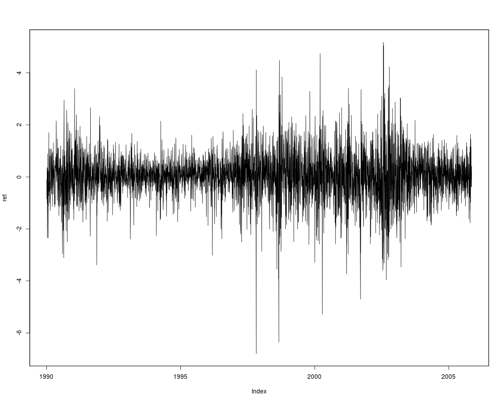
#############################################
## New York Stock Exchange composite index ##
#############################################
## returns
data("NYSESW", package = "AER")
ret <- 100 * diff(log(NYSESW))
plot(ret)
## fit GARCH(1,1)
library("tseries")
fm <- garch(coredata(ret))
Results
R version 3.3.1 (2016-06-21) -- "Bug in Your Hair"
Copyright (C) 2016 The R Foundation for Statistical Computing
Platform: x86_64-pc-linux-gnu (64-bit)

R is free software and comes with ABSOLUTELY NO WARRANTY.
You are welcome to redistribute it under certain conditions.
Type 'license()' or 'licence()' for distribution details.

R is a collaborative project with many contributors.
Type 'contributors()' for more information and
'citation()' on how to cite R or R packages in publications.

Type 'demo()' for some demos, 'help()' for on-line help, or
'help.start()' for an HTML browser interface to help.
Type 'q()' to quit R.

> library(AER)
Loading required package: car
Loading required package: lmtest
Loading required package: zoo

Attaching package: 'zoo'

The following objects are masked from 'package:base':

    as.Date, as.Date.numeric

Loading required package: sandwich
Loading required package: survival
> png(filename="/home/ddbj/snapshot/RGM3/R_CC/result/AER/StockWatson2007.Rd_%03d_medium.png", width=480, height=480)
> ### Name: StockWatson2007
> ### Title: Data and Examples from Stock and Watson (2007)
> ### Aliases: StockWatson2007
> ### Keywords: datasets
>
> ### ** Examples
>
> ###############################
> ## Current Population Survey ##
> ###############################
>
> ## p. 165
> data("CPSSWEducation", package = "AER")
> plot(earnings ~ education, data = CPSSWEducation)
> fm <- lm(earnings ~ education, data = CPSSWEducation)
> coeftest(fm, vcov = sandwich)

t test of coefficients:

             Estimate Std. Error t value  Pr(>|t|)
(Intercept) -3.134371   0.925571 -3.3864 0.0007174 ***
education    1.466925   0.071918 20.3972 < 2.2e-16 ***
---
Signif. codes:  0 '***' 0.001 '**' 0.01 '*' 0.05 '.' 0.1 ' ' 1

> abline(fm)
>
>
> ############################
> ## California test scores ##
> ############################
>
> ## data and transformations
> data("CASchools", package = "AER")
> CASchools$stratio <- with(CASchools, students/teachers)
> CASchools$score <- with(CASchools, (math + read)/2)
>
> ## p. 152
> fm1 <- lm(score ~ stratio, data = CASchools)
> coeftest(fm1, vcov = sandwich)

t test of coefficients:

             Estimate Std. Error t value  Pr(>|t|)
(Intercept) 698.93295   10.33966  67.597 < 2.2e-16 ***
stratio      -2.27981    0.51825  -4.399 1.382e-05 ***
---
Signif. codes:  0 '***' 0.001 '**' 0.01 '*' 0.05 '.' 0.1 ' ' 1

>
> ## p. 159
> fm2 <- lm(score ~ I(stratio < 20), data = CASchools)
> ## p. 199
> fm3 <- lm(score ~ stratio + english, data = CASchools)
> ## p. 224
> fm4 <- lm(score ~ stratio + expenditure + english, data = CASchools)
>
> ## Table 7.1, p. 242 (numbers refer to columns)
> fmc3 <- lm(score ~ stratio + english + lunch, data = CASchools)
> fmc4 <- lm(score ~ stratio + english + calworks, data = CASchools)
> fmc5 <- lm(score ~ stratio + english + lunch + calworks, data = CASchools)
>
> ## Equation 8.2, p. 258
> fmquad <- lm(score ~ income + I(income^2), data = CASchools)
> ## Equation 8.11, p. 266
> fmcub <- lm(score ~ income + I(income^2) + I(income^3), data = CASchools)
> ## Equation 8.23, p. 272
> fmloglog <- lm(log(score) ~ log(income), data = CASchools)
> ## Equation 8.24, p. 274
> fmloglin <- lm(log(score) ~ income, data = CASchools)
> ## Equation 8.26, p. 275
> fmlinlogcub <- lm(score ~ log(income) + I(log(income)^2) + I(log(income)^3),
+   data = CASchools)
>
> ## Table 8.3, p. 292 (numbers refer to columns)
> fmc2 <- lm(score ~ stratio + english + lunch + log(income), data = CASchools)
> fmc7 <- lm(score ~ stratio + I(stratio^2) + I(stratio^3) + english + lunch + log(income),
+   data = CASchools)
>
>
> #####################################
> ## Economics journal Subscriptions ##
> #####################################
>
> ## data and transformed variables
> data("Journals", package = "AER")
> journals <- Journals[, c("subs", "price")]
> journals$citeprice <- Journals$price/Journals$citations
> journals$age <- 2000 - Journals$foundingyear
> journals$chars <- Journals$charpp*Journals$pages/10^6
>
> ## Figure 8.9 (a) and (b)
> plot(subs ~ citeprice, data = journals, pch = 19)
> plot(log(subs) ~ log(citeprice), data = journals, pch = 19)
> fm1 <- lm(log(subs) ~ log(citeprice), data = journals)
> abline(fm1)
>
> ## Table 8.2, use HC1 for comparability with Stata
> fm1 <- lm(subs ~ citeprice, data = log(journals))
> fm2 <- lm(subs ~ citeprice + age + chars, data = log(journals))
> fm3 <- lm(subs ~ citeprice + I(citeprice^2) + I(citeprice^3) +
+   age + I(age * citeprice) + chars, data = log(journals))
> fm4 <- lm(subs ~ citeprice + age + I(age * citeprice) + chars, data = log(journals))
> coeftest(fm1, vcov = vcovHC(fm1, type = "HC1"))

t test of coefficients:

             Estimate Std. Error t value  Pr(>|t|)
(Intercept)  4.766212   0.055258  86.253 < 2.2e-16 ***
citeprice   -0.533053   0.033959 -15.697 < 2.2e-16 ***
---
Signif. codes:  0 '***' 0.001 '**' 0.01 '*' 0.05 '.' 0.1 ' ' 1

> coeftest(fm2, vcov = vcovHC(fm2, type = "HC1"))

t test of coefficients:

             Estimate Std. Error t value  Pr(>|t|)
(Intercept)  3.206648   0.379725  8.4447 1.102e-14 ***
citeprice   -0.407718   0.043717 -9.3262 < 2.2e-16 ***
age          0.423649   0.119064  3.5581 0.0004801 ***
chars        0.205614   0.097751  2.1035 0.0368474 *
---
Signif. codes:  0 '***' 0.001 '**' 0.01 '*' 0.05 '.' 0.1 ' ' 1

> coeftest(fm3, vcov = vcovHC(fm3, type = "HC1"))

t test of coefficients:

                     Estimate Std. Error t value  Pr(>|t|)
(Intercept)         3.4075956  0.3735992  9.1210 < 2.2e-16 ***
citeprice          -0.9609365  0.1601349 -6.0008 1.121e-08 ***
I(citeprice^2)      0.0165099  0.0254886  0.6477  0.518015
I(citeprice^3)      0.0036666  0.0055147  0.6649  0.507008
age                 0.3730539  0.1176966  3.1696  0.001805 **
I(age * citeprice)  0.1557773  0.0518947  3.0018  0.003081 **
chars               0.2346178  0.0977318  2.4006  0.017428 *
---
Signif. codes:  0 '***' 0.001 '**' 0.01 '*' 0.05 '.' 0.1 ' ' 1

> coeftest(fm4, vcov = vcovHC(fm4, type = "HC1"))

t test of coefficients:

                    Estimate Std. Error t value  Pr(>|t|)
(Intercept)         3.433521   0.367471  9.3436 < 2.2e-16 ***
citeprice          -0.898910   0.144648 -6.2144 3.656e-09 ***
age                 0.373515   0.117527  3.1781 0.0017529 **
I(age * citeprice)  0.140959   0.040199  3.5065 0.0005769 ***
chars               0.229466   0.096493  2.3781 0.0184822 *
---
Signif. codes:  0 '***' 0.001 '**' 0.01 '*' 0.05 '.' 0.1 ' ' 1

> waldtest(fm3, fm4, vcov = vcovHC(fm3, type = "HC1"))
Wald test

Model 1: subs ~ citeprice + I(citeprice^2) + I(citeprice^3) + age + I(age *
    citeprice) + chars
Model 2: subs ~ citeprice + age + I(age * citeprice) + chars
  Res.Df Df     F Pr(>F)
1    173
2    175 -2 0.249 0.7799
>
>
> ###############################
> ## Massachusetts test scores ##
> ###############################
>
> ## compare Massachusetts with California
> data("MASchools", package = "AER")
> data("CASchools", package = "AER")
> CASchools$stratio <- with(CASchools, students/teachers)
> CASchools$score4 <- with(CASchools, (math + read)/2)
>
> ## parts of Table 9.1, p. 330
> vars <- c("score4", "stratio", "english", "lunch", "income")
> cbind(
+   CA_mean = sapply(CASchools[, vars], mean),
+   CA_sd   = sapply(CASchools[, vars], sd),
+   MA_mean = sapply(MASchools[, vars], mean),
+   MA_sd   = sapply(MASchools[, vars], sd))
          CA_mean     CA_sd    MA_mean     MA_sd
score4  654.15655 19.053347 709.827273 15.126474
stratio  19.64043  1.891812  17.344091  2.276666
english  15.76816 18.285927   1.117676  2.900940
lunch    44.70524 27.123381  15.315909 15.060068
income   15.31659  7.225890  18.746764  5.807637
>
> ## Table 9.2, pp. 332--333, numbers refer to columns
> MASchools$higheng <- with(MASchools, english > median(english))
> fm1 <- lm(score4 ~ stratio, data = MASchools)
> fm2 <- lm(score4 ~ stratio + english + lunch + log(income), data = MASchools)
> fm3 <- lm(score4 ~ stratio + english + lunch + income + I(income^2) + I(income^3),
+   data = MASchools)
> fm4 <- lm(score4 ~ stratio + I(stratio^2) + I(stratio^3) + english + lunch +
+   income + I(income^2) + I(income^3), data = MASchools)
> fm5 <- lm(score4 ~ stratio + higheng + I(higheng * stratio) + lunch +
+   income + I(income^2) + I(income^3), data = MASchools)
> fm6 <- lm(score4 ~ stratio + lunch + income + I(income^2) + I(income^3),
+   data = MASchools)
>
> ## for comparability with Stata use HC1 below
> coeftest(fm1, vcov = vcovHC(fm1, type = "HC1"))

t test of coefficients:

             Estimate Std. Error t value  Pr(>|t|)
(Intercept) 739.62113    8.60727 85.9298 < 2.2e-16 ***
stratio      -1.71781    0.49906 -3.4421  0.000692 ***
---
Signif. codes:  0 '***' 0.001 '**' 0.01 '*' 0.05 '.' 0.1 ' ' 1

> coeftest(fm2, vcov = vcovHC(fm2, type = "HC1"))

t test of coefficients:

              Estimate Std. Error t value  Pr(>|t|)
(Intercept) 682.431602  11.497244 59.3561 < 2.2e-16 ***
stratio      -0.689179   0.269973 -2.5528   0.01138 *
english      -0.410745   0.306377 -1.3407   0.18145
lunch        -0.521465   0.077659 -6.7148 1.653e-10 ***
log(income)  16.529359   3.145722  5.2546 3.566e-07 ***
---
Signif. codes:  0 '***' 0.001 '**' 0.01 '*' 0.05 '.' 0.1 ' ' 1

> coeftest(fm3, vcov = vcovHC(fm3, type = "HC1"))

t test of coefficients:

               Estimate  Std. Error t value  Pr(>|t|)
(Intercept)  7.4403e+02  2.1318e+01 34.9016 < 2.2e-16 ***
stratio     -6.4091e-01  2.6848e-01 -2.3872   0.01785 *
english     -4.3712e-01  3.0332e-01 -1.4411   0.15103
lunch       -5.8182e-01  9.7353e-02 -5.9764 9.488e-09 ***
income      -3.0667e+00  2.3525e+00 -1.3036   0.19379
I(income^2)  1.6369e-01  8.5330e-02  1.9183   0.05641 .
I(income^3) -2.1793e-03  9.7033e-04 -2.2459   0.02574 *
---
Signif. codes:  0 '***' 0.001 '**' 0.01 '*' 0.05 '.' 0.1 ' ' 1

> coeftest(fm4, vcov = vcovHC(fm4, type = "HC1"))

t test of coefficients:

                Estimate  Std. Error t value  Pr(>|t|)
(Intercept)  665.4960529  81.3317629  8.1825 2.600e-14 ***
stratio       12.4259758  14.0101690  0.8869   0.37613
I(stratio^2)  -0.6803029   0.7365191 -0.9237   0.35671
I(stratio^3)   0.0114737   0.0126663  0.9058   0.36605
english       -0.4341659   0.2997883 -1.4482   0.14903
lunch         -0.5872165   0.1040207 -5.6452 5.283e-08 ***
income        -3.3815370   2.4906830 -1.3577   0.17602
I(income^2)    0.1741018   0.0892596  1.9505   0.05244 .
I(income^3)   -0.0022883   0.0010078 -2.2706   0.02418 *
---
Signif. codes:  0 '***' 0.001 '**' 0.01 '*' 0.05 '.' 0.1 ' ' 1

> coeftest(fm5, vcov = vcovHC(fm5, type = "HC1"))

t test of coefficients:

                        Estimate  Std. Error t value  Pr(>|t|)
(Intercept)          759.9142249  23.2331213 32.7082 < 2.2e-16 ***
stratio               -1.0176806   0.3703923 -2.7476  0.006521 **
highengTRUE          -12.5607339   9.7934588 -1.2826  0.201046
I(higheng * stratio)   0.7986123   0.5552225  1.4384  0.151805
lunch                 -0.7085098   0.0908442 -7.7992 2.785e-13 ***
income                -3.8665072   2.4884002 -1.5538  0.121721
I(income^2)            0.1841250   0.0898247  2.0498  0.041612 *
I(income^3)           -0.0023364   0.0010153 -2.3013  0.022349 *
---
Signif. codes:  0 '***' 0.001 '**' 0.01 '*' 0.05 '.' 0.1 ' ' 1

> coeftest(fm6, vcov = vcovHC(fm6, type = "HC1"))

t test of coefficients:

               Estimate  Std. Error t value Pr(>|t|)
(Intercept)  7.4736e+02  2.0278e+01 36.8563  < 2e-16 ***
stratio     -6.7188e-01  2.7128e-01 -2.4767  0.01404 *
lunch       -6.5308e-01  7.2980e-02 -8.9487  < 2e-16 ***
income      -3.2180e+00  2.3057e+00 -1.3956  0.16427
I(income^2)  1.6479e-01  8.4634e-02  1.9471  0.05284 .
I(income^3) -2.1550e-03  9.6995e-04 -2.2218  0.02735 *
---
Signif. codes:  0 '***' 0.001 '**' 0.01 '*' 0.05 '.' 0.1 ' ' 1

>
> ## Testing exclusion of groups of variables
> fm3r <- update(fm3, . ~ . - I(income^2) - I(income^3))
> waldtest(fm3, fm3r, vcov = vcovHC(fm3, type = "HC1"))
Wald test

Model 1: score4 ~ stratio + english + lunch + income + I(income^2) + I(income^3)
Model 2: score4 ~ stratio + english + lunch + income
  Res.Df Df      F    Pr(>F)
1    213
2    215 -2 7.7448 0.0005664 ***
---
Signif. codes:  0 '***' 0.001 '**' 0.01 '*' 0.05 '.' 0.1 ' ' 1
>
> fm4r_str1 <- update(fm4, . ~ . - stratio - I(stratio^2) - I(stratio^3))
> waldtest(fm4, fm4r_str1, vcov = vcovHC(fm4, type = "HC1"))
Wald test

Model 1: score4 ~ stratio + I(stratio^2) + I(stratio^3) + english + lunch +
    income + I(income^2) + I(income^3)
Model 2: score4 ~ english + lunch + income + I(income^2) + I(income^3)
  Res.Df Df      F  Pr(>F)
1    211
2    214 -3 2.8565 0.03809 *
---
Signif. codes:  0 '***' 0.001 '**' 0.01 '*' 0.05 '.' 0.1 ' ' 1
> fm4r_str2 <- update(fm4, . ~ . - I(stratio^2) - I(stratio^3))
> waldtest(fm4, fm4r_str2, vcov = vcovHC(fm4, type = "HC1"))
Wald test

Model 1: score4 ~ stratio + I(stratio^2) + I(stratio^3) + english + lunch +
    income + I(income^2) + I(income^3)
Model 2: score4 ~ stratio + english + lunch + income + I(income^2) + I(income^3)
  Res.Df Df      F Pr(>F)
1    211
2    213 -2 0.4463 0.6406
> fm4r_inc <- update(fm4, . ~ . - I(income^2) - I(income^3))
> waldtest(fm4, fm4r_inc, vcov = vcovHC(fm4, type = "HC1"))
Wald test

Model 1: score4 ~ stratio + I(stratio^2) + I(stratio^3) + english + lunch +
    income + I(income^2) + I(income^3)
Model 2: score4 ~ stratio + I(stratio^2) + I(stratio^3) + english + lunch +
    income
  Res.Df Df      F    Pr(>F)
1    211
2    213 -2 7.7487 0.0005657 ***
---
Signif. codes:  0 '***' 0.001 '**' 0.01 '*' 0.05 '.' 0.1 ' ' 1
>
> fm5r_str <- update(fm5, . ~ . - stratio - I(higheng * stratio))
> waldtest(fm5, fm5r_str, vcov = vcovHC(fm5, type = "HC1"))
Wald test

Model 1: score4 ~ stratio + higheng + I(higheng * stratio) + lunch + income +
    I(income^2) + I(income^3)
Model 2: score4 ~ higheng + lunch + income + I(income^2) + I(income^3)
  Res.Df Df      F Pr(>F)
1    212
2    214 -2 4.0062 0.0196 *
---
Signif. codes:  0 '***' 0.001 '**' 0.01 '*' 0.05 '.' 0.1 ' ' 1
> fm5r_inc <- update(fm5, . ~ . - I(income^2) - I(income^3))
> waldtest(fm5, fm5r_inc, vcov = vcovHC(fm5, type = "HC1"))
Wald test

Model 1: score4 ~ stratio + higheng + I(higheng * stratio) + lunch + income +
    I(income^2) + I(income^3)
Model 2: score4 ~ stratio + higheng + I(higheng * stratio) + lunch + income
  Res.Df Df      F   Pr(>F)
1    212
2    214 -2 5.8468 0.003375 **
---
Signif. codes:  0 '***' 0.001 '**' 0.01 '*' 0.05 '.' 0.1 ' ' 1
> fm5r_high <- update(fm5, . ~ . - higheng - I(higheng * stratio))
> waldtest(fm5, fm5r_high, vcov = vcovHC(fm5, type = "HC1"))
Wald test

Model 1: score4 ~ stratio + higheng + I(higheng * stratio) + lunch + income +
    I(income^2) + I(income^3)
Model 2: score4 ~ stratio + lunch + income + I(income^2) + I(income^3)
  Res.Df Df      F Pr(>F)
1    212
2    214 -2 1.5835 0.2077
>
> fm6r_inc <- update(fm6, . ~ . - I(income^2) - I(income^3))
> waldtest(fm6, fm6r_inc, vcov = vcovHC(fm6, type = "HC1"))
Wald test

Model 1: score4 ~ stratio + lunch + income + I(income^2) + I(income^3)
Model 2: score4 ~ stratio + lunch + income
  Res.Df Df      F   Pr(>F)
1    214
2    216 -2 6.5479 0.001737 **
---
Signif. codes:  0 '***' 0.001 '**' 0.01 '*' 0.05 '.' 0.1 ' ' 1
>
>
> ##################################
> ## Home mortgage disclosure act ##
> ##################################
>
> ## data
> data("HMDA", package = "AER")
>
> ## 11.1, 11.3, 11.7, 11.8 and 11.10, pp. 387--395
> fm1 <- lm(I(as.numeric(deny) - 1) ~ pirat, data = HMDA)
> fm2 <- lm(I(as.numeric(deny) - 1) ~ pirat + afam, data = HMDA)
> fm3 <- glm(deny ~ pirat, family = binomial(link = "probit"), data = HMDA)
> fm4 <- glm(deny ~ pirat + afam, family = binomial(link = "probit"), data = HMDA)
> fm5 <- glm(deny ~ pirat + afam, family = binomial(link = "logit"), data = HMDA)
>
> ## Table 11.1, p. 401
> mean(HMDA$pirat)
[1] 0.3308136
> mean(HMDA$hirat)
[1] 0.2553461
> mean(HMDA$lvrat)
[1] 0.7377759
> mean(as.numeric(HMDA$chist))
[1] 2.116387
> mean(as.numeric(HMDA$mhist))
[1] 1.721008
> mean(as.numeric(HMDA$phist)-1)
[1] 0.07352941
> prop.table(table(HMDA$insurance))

        no        yes
0.97983193 0.02016807
> prop.table(table(HMDA$selfemp))

       no       yes
0.8836134 0.1163866
> prop.table(table(HMDA$single))

       no       yes
0.6067227 0.3932773
> prop.table(table(HMDA$hschool))

        no        yes
0.01638655 0.98361345
> mean(HMDA$unemp)
[1] 3.774496
> prop.table(table(HMDA$condomin))

       no       yes
0.7117647 0.2882353
> prop.table(table(HMDA$afam))

      no      yes
0.857563 0.142437
> prop.table(table(HMDA$deny))

       no       yes
0.8802521 0.1197479
>
> ## Table 11.2, pp. 403--404, numbers refer to columns
> HMDA$lvrat <- factor(ifelse(HMDA$lvrat < 0.8, "low",
+   ifelse(HMDA$lvrat >= 0.8 & HMDA$lvrat <= 0.95, "medium", "high")),
+   levels = c("low", "medium", "high"))
> HMDA$mhist <- as.numeric(HMDA$mhist)
> HMDA$chist <- as.numeric(HMDA$chist)
>
> fm1 <- lm(I(as.numeric(deny) - 1) ~ afam + pirat + hirat + lvrat + chist + mhist +
+   phist + insurance + selfemp, data = HMDA)
> fm2 <- glm(deny ~ afam + pirat + hirat + lvrat + chist + mhist + phist + insurance +
+   selfemp, family = binomial, data = HMDA)
> fm3 <- glm(deny ~ afam + pirat + hirat + lvrat + chist + mhist + phist + insurance +
+   selfemp, family = binomial(link = "probit"), data = HMDA)
> fm4 <- glm(deny ~ afam + pirat + hirat + lvrat + chist + mhist + phist + insurance +
+   selfemp + single + hschool + unemp, family = binomial(link = "probit"), data = HMDA)
> fm5 <- glm(deny ~ afam + pirat + hirat + lvrat + chist + mhist + phist + insurance +
+   selfemp + single + hschool + unemp + condomin +
+   I(mhist==3) + I(mhist==4) + I(chist==3) + I(chist==4) + I(chist==5) + I(chist==6),
+   family = binomial(link = "probit"), data = HMDA)
> fm6 <- glm(deny ~ afam * (pirat + hirat) + lvrat + chist + mhist + phist + insurance +
+   selfemp + single + hschool + unemp, family = binomial(link = "probit"), data = HMDA)
> coeftest(fm1, vcov = sandwich)

t test of coefficients:

               Estimate Std. Error t value  Pr(>|t|)
(Intercept)  -0.1829933  0.0276089 -6.6281 4.197e-11 ***
afamyes       0.0836967  0.0225101  3.7182 0.0002053 ***
pirat         0.4487963  0.1133333  3.9600 7.717e-05 ***
hirat        -0.0480227  0.1093055 -0.4393 0.6604528
lvratmedium   0.0314498  0.0127097  2.4745 0.0134125 *
lvrathigh     0.1890511  0.0500520  3.7771 0.0001626 ***
chist         0.0307716  0.0045737  6.7279 2.150e-11 ***
mhist         0.0209104  0.0112637  1.8565 0.0635134 .
phistyes      0.1970876  0.0348005  5.6634 1.664e-08 ***
insuranceyes  0.7018841  0.0450008 15.5972 < 2.2e-16 ***
selfempyes    0.0598438  0.0204759  2.9227 0.0035035 **
---
Signif. codes:  0 '***' 0.001 '**' 0.01 '*' 0.05 '.' 0.1 ' ' 1

>
> fm4r <- update(fm4, . ~ . - single - hschool - unemp)
> waldtest(fm4, fm4r, vcov = sandwich)
Wald test

Model 1: deny ~ afam + pirat + hirat + lvrat + chist + mhist + phist +
    insurance + selfemp + single + hschool + unemp
Model 2: deny ~ afam + pirat + hirat + lvrat + chist + mhist + phist +
    insurance + selfemp
  Res.Df Df      F    Pr(>F)
1   2366
2   2369 -3 5.9463 0.0004893 ***
---
Signif. codes:  0 '***' 0.001 '**' 0.01 '*' 0.05 '.' 0.1 ' ' 1
> fm5r <- update(fm5, . ~ . - single - hschool - unemp)
> waldtest(fm5, fm5r, vcov = sandwich)
Wald test

Model 1: deny ~ afam + pirat + hirat + lvrat + chist + mhist + phist +
    insurance + selfemp + single + hschool + unemp + condomin +
    I(mhist == 3) + I(mhist == 4) + I(chist == 3) + I(chist ==
    4) + I(chist == 5) + I(chist == 6)
Model 2: deny ~ afam + pirat + hirat + lvrat + chist + mhist + phist +
    insurance + selfemp + condomin + I(mhist == 3) + I(mhist ==
    4) + I(chist == 3) + I(chist == 4) + I(chist == 5) + I(chist ==
    6)
  Res.Df Df      F   Pr(>F)
1   2359
2   2362 -3 5.1601 0.001482 **
---
Signif. codes:  0 '***' 0.001 '**' 0.01 '*' 0.05 '.' 0.1 ' ' 1
> fm6r <- update(fm6, . ~ . - single - hschool - unemp)
> waldtest(fm6, fm6r, vcov = sandwich)
Wald test

Model 1: deny ~ afam * (pirat + hirat) + lvrat + chist + mhist + phist +
    insurance + selfemp + single + hschool + unemp
Model 2: deny ~ afam + pirat + hirat + lvrat + chist + mhist + phist +
    insurance + selfemp + afam:pirat + afam:hirat
  Res.Df Df      F    Pr(>F)
1   2364
2   2367 -3 5.8876 0.0005316 ***
---
Signif. codes:  0 '***' 0.001 '**' 0.01 '*' 0.05 '.' 0.1 ' ' 1
>
> fm5r2 <- update(fm5, . ~ . - I(mhist==3) - I(mhist==4) - I(chist==3) - I(chist==4) -
+   I(chist==5) - I(chist==6))
> waldtest(fm5, fm5r2, vcov = sandwich)
Wald test

Model 1: deny ~ afam + pirat + hirat + lvrat + chist + mhist + phist +
    insurance + selfemp + single + hschool + unemp + condomin +
    I(mhist == 3) + I(mhist == 4) + I(chist == 3) + I(chist ==
    4) + I(chist == 5) + I(chist == 6)
Model 2: deny ~ afam + pirat + hirat + lvrat + chist + mhist + phist +
    insurance + selfemp + single + hschool + unemp + condomin
  Res.Df Df      F Pr(>F)
1   2359
2   2365 -6 1.2305 0.2873
>
> fm6r2 <- update(fm6, . ~ . - afam * (pirat + hirat) + pirat + hirat)
> waldtest(fm6, fm6r2, vcov = sandwich)
Wald test

Model 1: deny ~ afam * (pirat + hirat) + lvrat + chist + mhist + phist +
    insurance + selfemp + single + hschool + unemp
Model 2: deny ~ lvrat + chist + mhist + phist + insurance + selfemp +
    single + hschool + unemp + pirat + hirat
  Res.Df Df      F  Pr(>F)
1   2364
2   2367 -3 4.9217 0.00207 **
---
Signif. codes:  0 '***' 0.001 '**' 0.01 '*' 0.05 '.' 0.1 ' ' 1
>
> fm6r3 <- update(fm6, . ~ . - afam * (pirat + hirat) + pirat + hirat + afam)
> waldtest(fm6, fm6r3, vcov = sandwich)
Wald test

Model 1: deny ~ afam * (pirat + hirat) + lvrat + chist + mhist + phist +
    insurance + selfemp + single + hschool + unemp
Model 2: deny ~ lvrat + chist + mhist + phist + insurance + selfemp +
    single + hschool + unemp + pirat + hirat + afam
  Res.Df Df      F Pr(>F)
1   2364
2   2366 -2 0.2634 0.7685
>
>
>
> #########################################################
> ## Shooting down the "More Guns Less Crime" hypothesis ##
> #########################################################
>
> ## data
> data("Guns", package = "AER")
>
> ## Empirical Exercise 10.1
> fm1 <- lm(log(violent) ~ law, data = Guns)
> fm2 <- lm(log(violent) ~ law + prisoners + density + income +
+   population + afam + cauc + male, data = Guns)
> fm3 <- lm(log(violent) ~ law + prisoners + density + income +
+   population + afam + cauc + male + state, data = Guns)
> fm4 <- lm(log(violent) ~ law + prisoners + density + income +
+   population + afam + cauc + male + state + year, data = Guns)
> coeftest(fm1, vcov = sandwich)

t test of coefficients:

             Estimate Std. Error t value  Pr(>|t|)
(Intercept)  6.134919   0.019287 318.078 < 2.2e-16 ***
lawyes      -0.442965   0.047488  -9.328 < 2.2e-16 ***
---
Signif. codes:  0 '***' 0.001 '**' 0.01 '*' 0.05 '.' 0.1 ' ' 1

> coeftest(fm2, vcov = sandwich)

t test of coefficients:

               Estimate  Std. Error  t value  Pr(>|t|)
(Intercept)  2.9817e+00  6.0668e-01   4.9149 1.016e-06 ***
lawyes      -3.6839e-01  3.4654e-02 -10.6304 < 2.2e-16 ***
prisoners    1.6126e-03  1.8000e-04   8.9591 < 2.2e-16 ***
density      2.6688e-02  1.4294e-02   1.8671  0.062142 .
income       1.2051e-06  7.2498e-06   0.1662  0.868007
population   4.2710e-02  3.1345e-03  13.6255 < 2.2e-16 ***
afam         8.0853e-02  1.9916e-02   4.0598 5.241e-05 ***
cauc         3.1200e-02  9.6897e-03   3.2200  0.001317 **
male         8.8709e-03  1.2014e-02   0.7384  0.460435
---
Signif. codes:  0 '***' 0.001 '**' 0.01 '*' 0.05 '.' 0.1 ' ' 1

> printCoefmat(coeftest(fm3, vcov = sandwich)[1:9,])
               Estimate  Std. Error t value  Pr(>|t|)
(Intercept)  4.0368e+00  3.7479e-01 10.7708 < 2.2e-16 ***
lawyes      -4.6141e-02  1.9435e-02 -2.3741   0.01776 *
prisoners   -7.1008e-05  9.4831e-05 -0.7488   0.45414
density     -1.7229e-01  1.0221e-01 -1.6857   0.09213 .
income      -9.2037e-06  6.5619e-06 -1.4026   0.16102
population   1.1525e-02  9.4572e-03  1.2186   0.22325
afam         1.0428e-01  1.6133e-02  6.4636 1.526e-10 ***
cauc         4.0861e-02  5.2487e-03  7.7850 1.585e-14 ***
male        -5.0273e-02  7.5923e-03 -6.6215 5.518e-11 ***
---
Signif. codes:  0 '***' 0.001 '**' 0.01 '*' 0.05 '.' 0.1 ' ' 1
> printCoefmat(coeftest(fm4, vcov = sandwich)[1:9,])
               Estimate  Std. Error t value  Pr(>|t|)
(Intercept)  3.9720e+00  4.3322e-01  9.1685 < 2.2e-16 ***
lawyes      -2.7994e-02  1.8692e-02 -1.4976    0.1345
prisoners    7.5994e-05  8.0008e-05  0.9498    0.3424
density     -9.1555e-02  6.2588e-02 -1.4628    0.1438
income       9.5859e-07  6.9440e-06  0.1380    0.8902
population  -4.7545e-03  6.4673e-03 -0.7351    0.4624
afam         2.9186e-02  2.0298e-02  1.4379    0.1507
cauc         9.2500e-03  8.2188e-03  1.1255    0.2606
male         7.3326e-02  1.8116e-02  4.0475 5.542e-05 ***
---
Signif. codes:  0 '***' 0.001 '**' 0.01 '*' 0.05 '.' 0.1 ' ' 1
>
>
> ###########################
> ## US traffic fatalities ##
> ###########################
>
> ## data from Stock and Watson (2007)
> data("Fatalities")
> ## add fatality rate (number of traffic deaths
> ## per 10,000 people living in that state in that year)
> Fatalities$frate <- with(Fatalities, fatal/pop * 10000)
> ## add discretized version of minimum legal drinking age
> Fatalities$drinkagec <- cut(Fatalities$drinkage,
+   breaks = 18:22, include.lowest = TRUE, right = FALSE)
> Fatalities$drinkagec <- relevel(Fatalities$drinkagec, ref = 4)
> ## any punishment?
> Fatalities$punish <- with(Fatalities,
+   factor(jail == "yes" | service == "yes", labels = c("no", "yes")))
> ## plm package
> library("plm")
Loading required package: Formula
>
> ## for comparability with Stata we use HC1 below
> ## p. 351, Eq. (10.2)
> f1982 <- subset(Fatalities, year == "1982")
> fm_1982 <- lm(frate ~ beertax, data = f1982)
> coeftest(fm_1982, vcov = vcovHC(fm_1982, type = "HC1"))

t test of coefficients:

            Estimate Std. Error t value Pr(>|t|)
(Intercept)  2.01038    0.14957 13.4408   <2e-16 ***
beertax      0.14846    0.13261  1.1196   0.2687
---
Signif. codes:  0 '***' 0.001 '**' 0.01 '*' 0.05 '.' 0.1 ' ' 1

>
> ## p. 353, Eq. (10.3)
> f1988 <- subset(Fatalities, year == "1988")
> fm_1988 <- lm(frate ~ beertax, data = f1988)
> coeftest(fm_1988, vcov = vcovHC(fm_1988, type = "HC1"))

t test of coefficients:

            Estimate Std. Error t value  Pr(>|t|)
(Intercept)  1.85907    0.11461 16.2205 < 2.2e-16 ***
beertax      0.43875    0.12786  3.4314  0.001279 **
---
Signif. codes:  0 '***' 0.001 '**' 0.01 '*' 0.05 '.' 0.1 ' ' 1

>
> ## pp. 355, Eq. (10.8)
> fm_diff <- lm(I(f1988$frate - f1982$frate) ~ I(f1988$beertax - f1982$beertax))
> coeftest(fm_diff, vcov = vcovHC(fm_diff, type = "HC1"))

t test of coefficients:

                                  Estimate Std. Error t value Pr(>|t|)
(Intercept)                      -0.072037   0.065355 -1.1022 0.276091
I(f1988$beertax - f1982$beertax) -1.040973   0.355006 -2.9323 0.005229 **
---
Signif. codes:  0 '***' 0.001 '**' 0.01 '*' 0.05 '.' 0.1 ' ' 1

>
> ## pp. 360, Eq. (10.15)
> ##   (1) via formula
> fm_sfe <- lm(frate ~ beertax + state - 1, data = Fatalities)
> ##   (2) by hand
> fat <- with(Fatalities,
+   data.frame(frates = frate - ave(frate, state),
+   beertaxs = beertax - ave(beertax, state)))
> fm_sfe2 <- lm(frates ~ beertaxs - 1, data = fat)
> ##   (3) via plm()
> fm_sfe3 <- plm(frate ~ beertax, data = Fatalities,
+   index = c("state", "year"), model = "within")
>
> coeftest(fm_sfe, vcov = vcovHC(fm_sfe, type = "HC1"))[1,]
    Estimate   Std. Error      t value     Pr(>|t|)
-0.655873722  0.203279719 -3.226459220  0.001398372
>
> ## uses different df in sd and p-value
> coeftest(fm_sfe2, vcov = vcovHC(fm_sfe2, type = "HC1"))[1,]
    Estimate   Std. Error      t value     Pr(>|t|)
-0.655873722  0.188153627 -3.485841496  0.000555894
>
> ## uses different df in p-value
> coeftest(fm_sfe3, vcov = vcovHC(fm_sfe3, type = "HC1", method = "white1"))[1,]
     Estimate    Std. Error       t value      Pr(>|t|)
-0.6558737222  0.1881536274 -3.4858414958  0.0005673213
>
>
> ## pp. 363, Eq. (10.21)
> ## via lm()
> fm_stfe <- lm(frate ~ beertax + state + year - 1, data = Fatalities)
> coeftest(fm_stfe, vcov = vcovHC(fm_stfe, type = "HC1"))[1,]
  Estimate Std. Error    t value   Pr(>|t|)
-0.6399800  0.2547149 -2.5125346  0.0125470
> ## via plm()
> fm_stfe2 <- plm(frate ~ beertax, data = Fatalities,
+   index = c("state", "year"), model = "within", effect = "twoways")
> coeftest(fm_stfe2, vcov = vcovHC) ## different

t test of coefficients:

        Estimate Std. Error t value Pr(>|t|)
beertax -0.63998    0.34963 -1.8305  0.06824 .
---
Signif. codes:  0 '***' 0.001 '**' 0.01 '*' 0.05 '.' 0.1 ' ' 1

>
>
> ## p. 368, Table 10.1, numbers refer to cols.
> fm1 <- plm(frate ~ beertax, data = Fatalities, index = c("state", "year"),
+   model = "pooling")
> fm2 <- plm(frate ~ beertax, data = Fatalities, index = c("state", "year"),
+   model = "within")
> fm3 <- plm(frate ~ beertax, data = Fatalities, index = c("state", "year"),
+   model = "within", effect = "twoways")
> fm4 <- plm(frate ~ beertax + drinkagec + jail + service + miles + unemp + log(income),
+   data = Fatalities, index = c("state", "year"), model = "within", effect = "twoways")
> fm
|