US Consumption Data (1940–1950)

Description

Time series data on US income and consumption expenditure, 1940–1950.

Usage

data("USConsump1950")

Format

An annual multiple time series from 1940 to 1950 with 3 variables.

income

Disposable income.

expenditure

Consumption expenditure.

war

Indicator variable: Was the year a year of war?

Source

Online complements to Greene (2003). Table F2.1.

http://pages.stern.nyu.edu/~wgreene/Text/tables/tablelist5.htm

References

Greene, W.H. (2003). Econometric Analysis, 5th edition. Upper Saddle River, NJ: Prentice Hall.

See Also

Greene2003, USConsump1979, USConsump1993

Examples

## Greene (2003)
## data
data("USConsump1950")
usc <- as.data.frame(USConsump1950)
usc$war <- factor(usc$war, labels = c("no", "yes"))

## Example 2.1
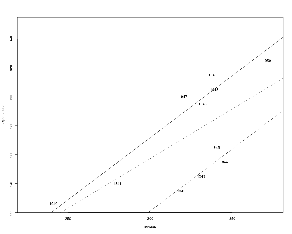
plot(expenditure ~ income, data = usc, type = "n", xlim = c(225, 375), ylim = c(225, 350))
with(usc, text(income, expenditure, time(USConsump1950)))

## single model
fm <- lm(expenditure ~ income, data = usc)
summary(fm)

## different intercepts for war yes/no
fm2 <- lm(expenditure ~ income + war, data = usc)
summary(fm2)

## compare
anova(fm, fm2)

## visualize
abline(fm, lty = 3)                                   
abline(coef(fm2)[1:2])                                
abline(sum(coef(fm2)[c(1, 3)]), coef(fm2)[2], lty = 2)

## Example 3.2
summary(fm)$r.squared
summary(lm(expenditure ~ income, data = usc, subset = war == "no"))$r.squared
summary(fm2)$r.squared

Results

R version 3.3.1 (2016-06-21) -- "Bug in Your Hair"
Copyright (C) 2016 The R Foundation for Statistical Computing
Platform: x86_64-pc-linux-gnu (64-bit)

R is free software and comes with ABSOLUTELY NO WARRANTY.
You are welcome to redistribute it under certain conditions.
Type 'license()' or 'licence()' for distribution details.

R is a collaborative project with many contributors.
Type 'contributors()' for more information and
'citation()' on how to cite R or R packages in publications.

Type 'demo()' for some demos, 'help()' for on-line help, or
'help.start()' for an HTML browser interface to help.
Type 'q()' to quit R.

> library(AER)
Loading required package: car
Loading required package: lmtest
Loading required package: zoo

Attaching package: 'zoo'

The following objects are masked from 'package:base':

    as.Date, as.Date.numeric

Loading required package: sandwich
Loading required package: survival
> png(filename="/home/ddbj/snapshot/RGM3/R_CC/result/AER/USConsump1950.Rd_%03d_medium.png", width=480, height=480)
> ### Name: USConsump1950
> ### Title: US Consumption Data (1940-1950)
> ### Aliases: USConsump1950
> ### Keywords: datasets
> 
> ### ** Examples
> 
> ## Greene (2003)
> ## data
> data("USConsump1950")
> usc <- as.data.frame(USConsump1950)
> usc$war <- factor(usc$war, labels = c("no", "yes"))
> 
> ## Example 2.1
> plot(expenditure ~ income, data = usc, type = "n", xlim = c(225, 375), ylim = c(225, 350))
> with(usc, text(income, expenditure, time(USConsump1950)))
> 
> ## single model
> fm <- lm(expenditure ~ income, data = usc)
> summary(fm)

Call:
lm(formula = expenditure ~ income, data = usc)

Residuals:
    Min      1Q  Median      3Q     Max 
-35.347 -26.440   9.068  20.000  31.642 

Coefficients:
            Estimate Std. Error t value Pr(>|t|)  
(Intercept)  51.8951    80.8440   0.642   0.5369  
income        0.6848     0.2488   2.753   0.0224 *
---
Signif. codes:  0 '***' 0.001 '**' 0.01 '*' 0.05 '.' 0.1 ' ' 1

Residual standard error: 27.59 on 9 degrees of freedom
Multiple R-squared:  0.4571,	Adjusted R-squared:  0.3968 
F-statistic: 7.579 on 1 and 9 DF,  p-value: 0.02237

> 
> ## different intercepts for war yes/no
> fm2 <- lm(expenditure ~ income + war, data = usc)
> summary(fm2)

Call:
lm(formula = expenditure ~ income + war, data = usc)

Residuals:
    Min      1Q  Median      3Q     Max 
-14.598  -4.418  -2.352   7.242  11.101 

Coefficients:
             Estimate Std. Error t value Pr(>|t|)    
(Intercept)  14.49540   27.29948   0.531     0.61    
income        0.85751    0.08534  10.048 8.19e-06 ***
waryes      -50.68974    5.93237  -8.545 2.71e-05 ***
---
Signif. codes:  0 '***' 0.001 '**' 0.01 '*' 0.05 '.' 0.1 ' ' 1

Residual standard error: 9.195 on 8 degrees of freedom
Multiple R-squared:  0.9464,	Adjusted R-squared:  0.933 
F-statistic: 70.61 on 2 and 8 DF,  p-value: 8.26e-06

> 
> ## compare
> anova(fm, fm2)
Analysis of Variance Table

Model 1: expenditure ~ income
Model 2: expenditure ~ income + war
  Res.Df    RSS Df Sum of Sq     F   Pr(>F)    
1      9 6850.0                                
2      8  676.5  1    6173.5 73.01 2.71e-05 ***
---
Signif. codes:  0 '***' 0.001 '**' 0.01 '*' 0.05 '.' 0.1 ' ' 1
> 
> ## visualize
> abline(fm, lty = 3)                                   
> abline(coef(fm2)[1:2])                                
> abline(sum(coef(fm2)[c(1, 3)]), coef(fm2)[2], lty = 2)
> 
> ## Example 3.2
> summary(fm)$r.squared
[1] 0.4571345
> summary(lm(expenditure ~ income, data = usc, subset = war == "no"))$r.squared
[1] 0.9369742
> summary(fm2)$r.squared
[1] 0.9463904
> 
> 
> 
> 
> 
> dev.off()
null device 
          1 
>