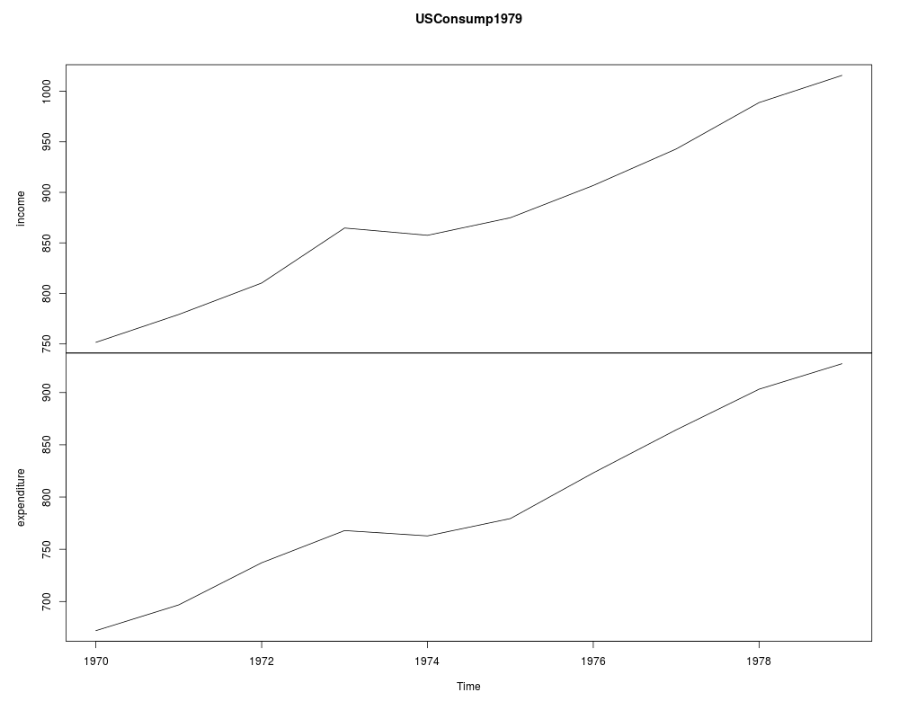
US Consumption Data (1970–1979)

Description

Time series data on US income and consumption expenditure, 1970–1979.

Usage

data("USConsump1979")

Format

An annual multiple time series from 1970 to 1979 with 2 variables.

income

Disposable income.

expenditure

Consumption expenditure.

Source

Online complements to Greene (2003). Table F1.1.

http://pages.stern.nyu.edu/~wgreene/Text/tables/tablelist5.htm

References

Greene, W.H. (2003). Econometric Analysis, 5th edition. Upper Saddle River, NJ: Prentice Hall.

See Also

Greene2003, USConsump1950, USConsump1993

Examples

data("USConsump1979")
plot(USConsump1979)

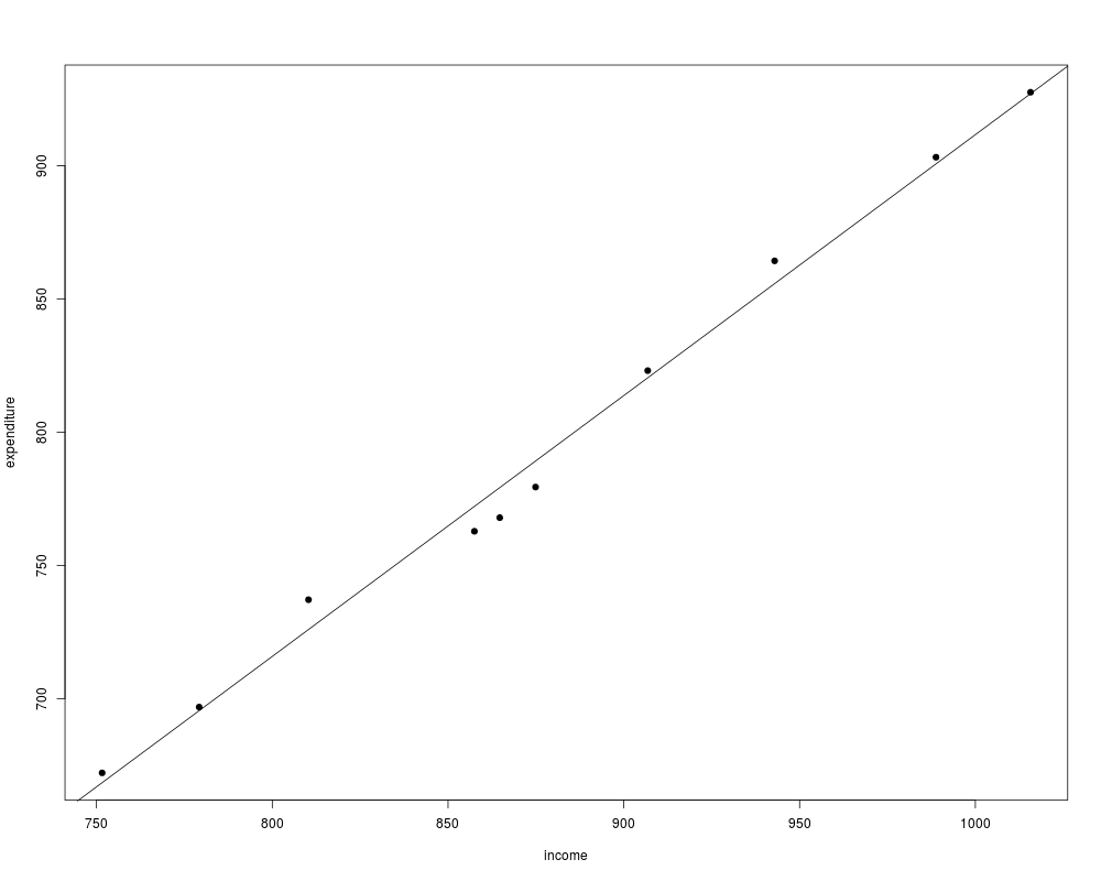
## Example 1.1 in Greene (2003)
plot(expenditure ~ income, data = as.data.frame(USConsump1979), pch = 19)
fm <- lm(expenditure ~ income, data = as.data.frame(USConsump1979))
summary(fm)
abline(fm)

Results

R version 3.3.1 (2016-06-21) -- "Bug in Your Hair"
Copyright (C) 2016 The R Foundation for Statistical Computing
Platform: x86_64-pc-linux-gnu (64-bit)

R is free software and comes with ABSOLUTELY NO WARRANTY.
You are welcome to redistribute it under certain conditions.
Type 'license()' or 'licence()' for distribution details.

R is a collaborative project with many contributors.
Type 'contributors()' for more information and
'citation()' on how to cite R or R packages in publications.

Type 'demo()' for some demos, 'help()' for on-line help, or
'help.start()' for an HTML browser interface to help.
Type 'q()' to quit R.

> library(AER)
Loading required package: car
Loading required package: lmtest
Loading required package: zoo

Attaching package: 'zoo'

The following objects are masked from 'package:base':

    as.Date, as.Date.numeric

Loading required package: sandwich
Loading required package: survival
> png(filename="/home/ddbj/snapshot/RGM3/R_CC/result/AER/USConsump1979.Rd_%03d_medium.png", width=480, height=480)
> ### Name: USConsump1979
> ### Title: US Consumption Data (1970-1979)
> ### Aliases: USConsump1979
> ### Keywords: datasets
> 
> ### ** Examples
> 
> data("USConsump1979")
> plot(USConsump1979)
> 
> ## Example 1.1 in Greene (2003)
> plot(expenditure ~ income, data = as.data.frame(USConsump1979), pch = 19)
> fm <- lm(expenditure ~ income, data = as.data.frame(USConsump1979))
> summary(fm)

Call:
lm(formula = expenditure ~ income, data = as.data.frame(USConsump1979))

Residuals:
    Min      1Q  Median      3Q     Max 
-11.291  -6.871   1.909   3.418  11.181 

Coefficients:
             Estimate Std. Error t value Pr(>|t|)    
(Intercept) -67.58065   27.91071  -2.421   0.0418 *  
income        0.97927    0.03161  30.983 1.28e-09 ***
---
Signif. codes:  0 '***' 0.001 '**' 0.01 '*' 0.05 '.' 0.1 ' ' 1

Residual standard error: 8.193 on 8 degrees of freedom
Multiple R-squared:  0.9917,	Adjusted R-squared:  0.9907 
F-statistic: 959.9 on 1 and 8 DF,  p-value: 1.28e-09

> abline(fm)
> 
> 
> 
> 
> 
> dev.off()
null device 
          1 
>