Supported by Dr. Osamu Ogasawara and  . . |
|
Last data update: 2014.03.03 |
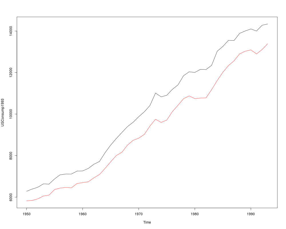
US Consumption Data (1950–1993)DescriptionTime series data on US income and consumption expenditure, 1950–1993. Usagedata("USConsump1993")
FormatAn annual multiple time series from 1950 to 1993 with 2 variables.
SourceThe data is from Baltagi (2002). ReferencesBaltagi, B.H. (2002). Econometrics, 3rd ed. Berlin, Springer. See Also
Examples
## data from Baltagi (2002)
data("USConsump1993", package = "AER")
plot(USConsump1993, plot.type = "single", col = 1:2)
## Chapter 5 (p. 122-125)
fm <- lm(expenditure ~ income, data = USConsump1993)
summary(fm)
## Durbin-Watson test (p. 122)
dwtest(fm)
## Breusch-Godfrey test (Table 5.4, p. 124)
bgtest(fm)
## Newey-West standard errors (Table 5.5, p. 125)
coeftest(fm, vcov = NeweyWest(fm, lag = 3, prewhite = FALSE, adjust = TRUE))
## Chapter 8
library("strucchange")
## Recursive residuals
rr <- recresid(fm)
rr
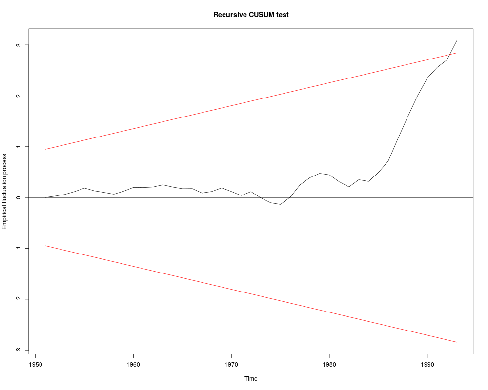
## Recursive CUSUM test
rcus <- efp(expenditure ~ income, data = USConsump1993)
plot(rcus)
sctest(rcus)
## Harvey-Collier test
harvtest(fm)
## NOTE" Mistake in Baltagi (2002) who computes
## the t-statistic incorrectly as 0.0733 via
mean(rr)/sd(rr)/sqrt(length(rr))
## whereas it should be (as in harvtest)
mean(rr)/sd(rr) * sqrt(length(rr))
## Rainbow test
raintest(fm, center = 23)
## J test for non-nested models
library("dynlm")
fm1 <- dynlm(expenditure ~ income + L(income), data = USConsump1993)
fm2 <- dynlm(expenditure ~ income + L(expenditure), data = USConsump1993)
jtest(fm1, fm2)
## Chapter 14
## ACF and PACF for expenditures and first differences
exps <- USConsump1993[, "expenditure"]
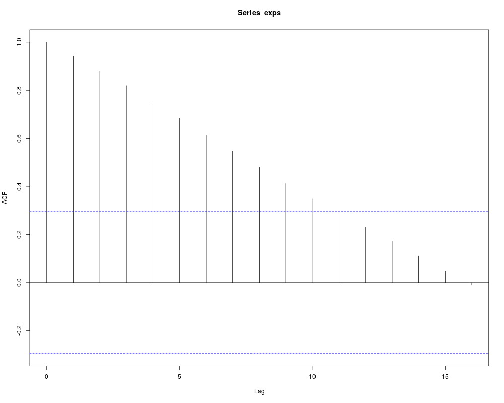
(acf(exps))
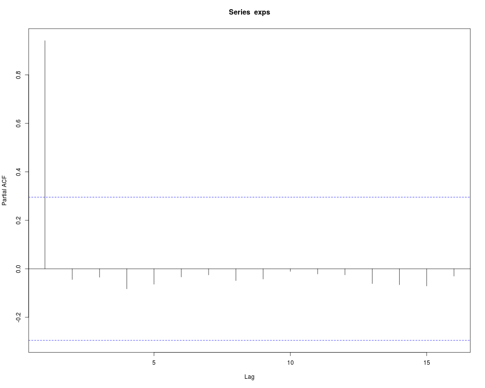
(pacf(exps))
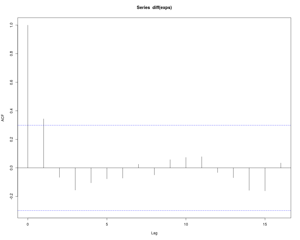
(acf(diff(exps)))
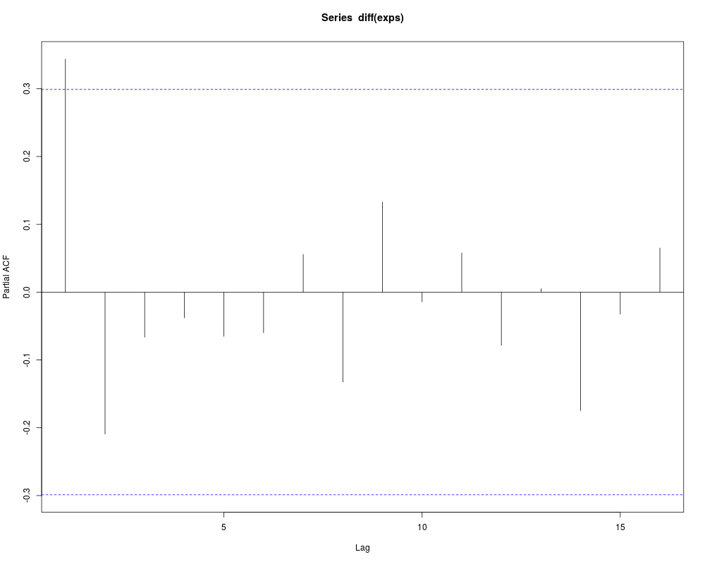
(pacf(diff(exps)))
## dynamic regressions, eq. (14.8)
fm <- dynlm(d(exps) ~ I(time(exps) - 1949) + L(exps))
summary(fm)
Results
R version 3.3.1 (2016-06-21) -- "Bug in Your Hair"
Copyright (C) 2016 The R Foundation for Statistical Computing
Platform: x86_64-pc-linux-gnu (64-bit)

R is free software and comes with ABSOLUTELY NO WARRANTY.
You are welcome to redistribute it under certain conditions.
Type 'license()' or 'licence()' for distribution details.

R is a collaborative project with many contributors.
Type 'contributors()' for more information and
'citation()' on how to cite R or R packages in publications.

Type 'demo()' for some demos, 'help()' for on-line help, or
'help.start()' for an HTML browser interface to help.
Type 'q()' to quit R.

> library(AER)
Loading required package: car
Loading required package: lmtest
Loading required package: zoo

Attaching package: 'zoo'

The following objects are masked from 'package:base':

    as.Date, as.Date.numeric

Loading required package: sandwich
Loading required package: survival
> png(filename="/home/ddbj/snapshot/RGM3/R_CC/result/AER/USConsump1993.Rd_%03d_medium.png", width=480, height=480)
> ### Name: USConsump1993
> ### Title: US Consumption Data (1950-1993)
> ### Aliases: USConsump1993
> ### Keywords: datasets
>
> ### ** Examples
>
> ## data from Baltagi (2002)
> data("USConsump1993", package = "AER")
> plot(USConsump1993, plot.type = "single", col = 1:2)
>
> ## Chapter 5 (p. 122-125)
> fm <- lm(expenditure ~ income, data = USConsump1993)
> summary(fm)

Call:
lm(formula = expenditure ~ income, data = USConsump1993)

Residuals:
    Min      1Q  Median      3Q     Max
-294.52  -67.02    4.64   90.02  325.84

Coefficients:
              Estimate Std. Error t value Pr(>|t|)
(Intercept) -65.795821  90.990824  -0.723    0.474
income        0.915623   0.008648 105.874   <2e-16 ***
---
Signif. codes:  0 '***' 0.001 '**' 0.01 '*' 0.05 '.' 0.1 ' ' 1

Residual standard error: 153.6 on 42 degrees of freedom
Multiple R-squared:  0.9963,	Adjusted R-squared:  0.9962
F-statistic: 1.121e+04 on 1 and 42 DF,  p-value: < 2.2e-16

> ## Durbin-Watson test (p. 122)
> dwtest(fm)

	Durbin-Watson test

data:  fm
DW = 0.46078, p-value = 3.274e-11
alternative hypothesis: true autocorrelation is greater than 0

> ## Breusch-Godfrey test (Table 5.4, p. 124)
> bgtest(fm)

	Breusch-Godfrey test for serial correlation of order up to 1

data:  fm
LM test = 24.901, df = 1, p-value = 6.034e-07

> ## Newey-West standard errors (Table 5.5, p. 125)
> coeftest(fm, vcov = NeweyWest(fm, lag = 3, prewhite = FALSE, adjust = TRUE))

t test of coefficients:

              Estimate Std. Error t value Pr(>|t|)
(Intercept) -65.795821 133.345400 -0.4934   0.6243
income        0.915623   0.015458 59.2319   <2e-16 ***
---
Signif. codes:  0 '***' 0.001 '**' 0.01 '*' 0.05 '.' 0.1 ' ' 1

>
> ## Chapter 8
> library("strucchange")
> ## Recursive residuals
> rr <- recresid(fm)
> rr
 [1]   24.900681   30.354827   50.893291   63.260389  -49.805907  -28.404311
 [7]  -31.520559   53.194256   67.696114   -2.646556    9.679147   39.658827
[13]  -40.126557  -30.260756    2.605633  -78.941467   27.185066   64.363195
[19]  -64.906717  -71.641013   70.095867 -113.475323  -85.633171  -29.427630
[25]  128.328459  220.693133  126.591749   78.394247  -25.955574 -124.178686
[31]  -90.845193  127.830581  -30.794629  159.780872  201.707127  405.310561
[37]  390.953841  373.370919  316.431235  188.109683  134.461285  339.300414
> ## Recursive CUSUM test
> rcus <- efp(expenditure ~ income, data = USConsump1993)
> plot(rcus)
> sctest(rcus)

	Recursive CUSUM test

data:  rcus
S = 1.0267, p-value = 0.02707

> ## Harvey-Collier test
> harvtest(fm)

	Harvey-Collier test

data:  fm
HC = 3.0802, df = 41, p-value = 0.003685

> ## NOTE" Mistake in Baltagi (2002) who computes
> ## the t-statistic incorrectly as 0.0733 via
> mean(rr)/sd(rr)/sqrt(length(rr))
[1] 0.07333754
> ## whereas it should be (as in harvtest)
> mean(rr)/sd(rr) * sqrt(length(rr))
[1] 3.080177
>
> ## Rainbow test
> raintest(fm, center = 23)

	Rainbow test

data:  fm
Rain = 4.1448, df1 = 22, df2 = 20, p-value = 0.001116

>
> ## J test for non-nested models
> library("dynlm")
> fm1 <- dynlm(expenditure ~ income + L(income), data = USConsump1993)
> fm2 <- dynlm(expenditure ~ income + L(expenditure), data = USConsump1993)
> jtest(fm1, fm2)
J test

Model 1: expenditure ~ income + L(income)
Model 2: expenditure ~ income + L(expenditure)
                Estimate Std. Error t value  Pr(>|t|)
M1 + fitted(M2)   1.6378    0.20984  7.8051 1.726e-09 ***
M2 + fitted(M1)  -2.5419    0.61603 -4.1262 0.0001874 ***
---
Signif. codes:  0 '***' 0.001 '**' 0.01 '*' 0.05 '.' 0.1 ' ' 1
>
> ## Chapter 14
> ## ACF and PACF for expenditures and first differences
> exps <- USConsump1993[, "expenditure"]
> (acf(exps))

Autocorrelations of series 'exps', by lag

     0      1      2      3      4      5      6      7      8      9     10
 1.000  0.941  0.880  0.820  0.753  0.683  0.614  0.547  0.479  0.412  0.348
    11     12     13     14     15     16
 0.288  0.230  0.171  0.110  0.049 -0.010
> (pacf(exps))

Partial autocorrelations of series 'exps', by lag

     1      2      3      4      5      6      7      8      9     10     11
 0.941 -0.045 -0.035 -0.083 -0.064 -0.034 -0.025 -0.049 -0.043 -0.011 -0.022
    12     13     14     15     16
-0.025 -0.061 -0.066 -0.071 -0.030
> (acf(diff(exps)))

Autocorrelations of series 'diff(exps)', by lag

     0      1      2      3      4      5      6      7      8      9     10
 1.000  0.344 -0.067 -0.156 -0.105 -0.077 -0.072  0.026 -0.050  0.058  0.073
    11     12     13     14     15     16
 0.078 -0.033 -0.069 -0.158 -0.161  0.034
> (pacf(diff(exps)))

Partial autocorrelations of series 'diff(exps)', by lag

     1      2      3      4      5      6      7      8      9     10     11
 0.344 -0.209 -0.066 -0.038 -0.065 -0.060  0.056 -0.133  0.133 -0.014  0.058
    12     13     14     15     16
-0.079  0.005 -0.175 -0.032  0.065
>
> ## dynamic regressions, eq. (14.8)
> fm <- dynlm(d(exps) ~ I(time(exps) - 1949) + L(exps))
> summary(fm)

Time series regression with "ts" data:
Start = 1951, End = 1993

Call:
dynlm(formula = d(exps) ~ I(time(exps) - 1949) + L(exps))

Residuals:
    Min      1Q  Median      3Q     Max
-357.76  -78.18   22.49  108.97  201.06

Coefficients:
                       Estimate Std. Error t value Pr(>|t|)
(Intercept)          1048.96039  353.81291   2.965  0.00509 **
I(time(exps) - 1949)   39.90164   14.31344   2.788  0.00808 **
L(exps)                -0.19561    0.07398  -2.644  0.01164 *
---
Signif. codes:  0 '***' 0.001 '**' 0.01 '*' 0.05 '.' 0.1 ' ' 1

Residual standard error: 147.4 on 40 degrees of freedom
Multiple R-squared:  0.1784,	Adjusted R-squared:  0.1373
F-statistic: 4.343 on 2 and 40 DF,  p-value: 0.01963

>
>
>
>
>
> dev.off()
null device
          1
>
|
Created & Maintained by Osamu Ogasawara (osamu.ogasawara@gmail.com) and 