Supported by Dr. Osamu Ogasawara and  . . |
|
Last data update: 2014.03.03 |
Data and Examples from Winkelmann and Boes (2009)DescriptionThis manual page collects a list of examples from the book. Some solutions might not be exact and the list is not complete. If you have suggestions for improvement (preferably in the form of code), please contact the package maintainer. ReferencesWinkelmann, R., and Boes, S. (2009). Analysis of Microdata, 2nd ed. Berlin and Heidelberg: Springer-Verlag. See Also
Examples
#########################################
## US General Social Survey 1974--2002 ##
#########################################
## data
data("GSS7402", package = "AER")
## completed fertility subset
gss40 <- subset(GSS7402, age >= 40)
## Chapter 1
## Table 1.1
gss_kids <- table(gss40$kids)
cbind(absolute = gss_kids,
relative = round(prop.table(gss_kids) * 100, digits = 2))
## Table 1.2
sd1 <- function(x) sd(x) / sqrt(length(x))
with(gss40, round(cbind(
"obs" = tapply(kids, year, length),
"av kids" = tapply(kids, year, mean),
" " = tapply(kids, year, sd1),
"prop childless" = tapply(kids, year, function(x) mean(x <= 0)),
" " = tapply(kids, year, function(x) sd1(x <= 0)),
"av schooling" = tapply(education, year, mean),
" " = tapply(education, year, sd1)
), digits = 2))
## Table 1.3
gss40$trend <- gss40$year - 1974
kids_lm1 <- lm(kids ~ factor(year), data = gss40)
kids_lm2 <- lm(kids ~ trend, data = gss40)
kids_lm3 <- lm(kids ~ trend + education, data = gss40)
## Chapter 2
## Table 2.1
kids_tab <- prop.table(xtabs(~ kids + year, data = gss40), 2) * 100
round(kids_tab[,c(4, 8)], digits = 2)
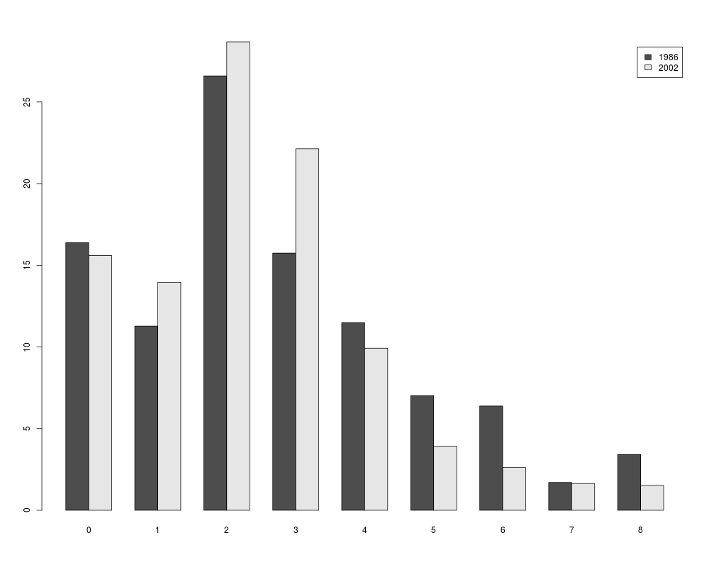
## Figure 2.1
barplot(t(kids_tab[, c(4, 8)]), beside = TRUE, legend = TRUE)
## Chapter 3, Example 3.14
## Table 3.1
gss40$nokids <- factor(gss40$kids <= 0,
levels = c(FALSE, TRUE), labels = c("no", "yes"))
nokids_p1 <- glm(nokids ~ 1, data = gss40, family = binomial(link = "probit"))
nokids_p2 <- glm(nokids ~ trend, data = gss40, family = binomial(link = "probit"))
nokids_p3 <- glm(nokids ~ trend + education + ethnicity + siblings,
data = gss40, family = binomial(link = "probit"))
## p. 87
lrtest(nokids_p1, nokids_p2, nokids_p3)
## Chapter 4, Example 4.1
gss40$nokids01 <- as.numeric(gss40$nokids) - 1
nokids_lm3 <- lm(nokids01 ~ trend + education + ethnicity + siblings, data = gss40)
coeftest(nokids_lm3, vcov = sandwich)
## Example 4.3
## Table 4.1
nokids_l1 <- glm(nokids ~ 1, data = gss40, family = binomial(link = "logit"))
nokids_l3 <- glm(nokids ~ trend + education + ethnicity + siblings,
data = gss40, family = binomial(link = "logit"))
lrtest(nokids_p3)
lrtest(nokids_l3)
## Table 4.2
nokids_xbar <- colMeans(model.matrix(nokids_l3))
sum(coef(nokids_p3) * nokids_xbar)
sum(coef(nokids_l3) * nokids_xbar)
dnorm(sum(coef(nokids_p3) * nokids_xbar))
dlogis(sum(coef(nokids_l3) * nokids_xbar))
dnorm(sum(coef(nokids_p3) * nokids_xbar)) * coef(nokids_p3)[3]
dlogis(sum(coef(nokids_l3) * nokids_xbar)) * coef(nokids_l3)[3]
exp(coef(nokids_l3)[3])
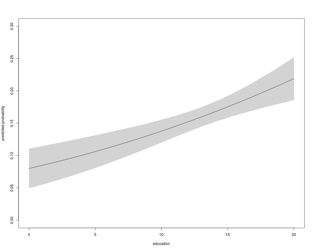
## Figure 4.4
## everything by hand (for ethnicity = "cauc" group)
nokids_xbar <- as.vector(nokids_xbar)
nokids_nd <- data.frame(education = seq(0, 20, by = 0.5), trend = nokids_xbar[2],
ethnicity = "cauc", siblings = nokids_xbar[4])
nokids_p3_fit <- predict(nokids_p3, newdata = nokids_nd,
type = "response", se.fit = TRUE)
plot(nokids_nd$education, nokids_p3_fit$fit, type = "l",
xlab = "education", ylab = "predicted probability", ylim = c(0, 0.3))
polygon(c(nokids_nd$education, rev(nokids_nd$education)),
c(nokids_p3_fit$fit + 1.96 * nokids_p3_fit$se.fit,
rev(nokids_p3_fit$fit - 1.96 * nokids_p3_fit$se.fit)),
col = "lightgray", border = "lightgray")
lines(nokids_nd$education, nokids_p3_fit$fit)
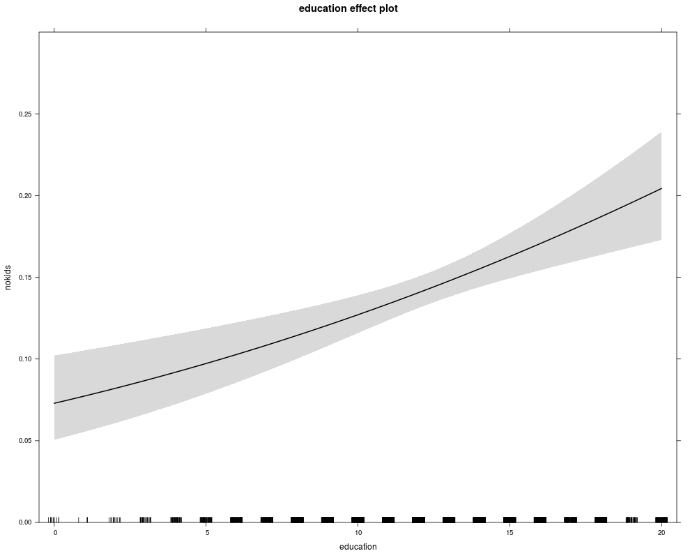
## using "effects" package (for average "ethnicity" variable)
library("effects")
nokids_p3_ef <- effect("education", nokids_p3, xlevels = list(education = 0:20))
plot(nokids_p3_ef, rescale.axis = FALSE, ylim = c(0, 0.3))
## using "effects" plus modification by hand
nokids_p3_ef1 <- as.data.frame(nokids_p3_ef)
plot(pnorm(fit) ~ education, data = nokids_p3_ef1, type = "n", ylim = c(0, 0.3))
polygon(c(0:20, 20:0), pnorm(c(nokids_p3_ef1$upper, rev(nokids_p3_ef1$lower))),
col = "lightgray", border = "lightgray")
lines(pnorm(fit) ~ education, data = nokids_p3_ef1)
## Table 4.6
## McFadden's R^2
1 - as.numeric( logLik(nokids_p3) / logLik(nokids_p1) )
1 - as.numeric( logLik(nokids_l3) / logLik(nokids_l1) )
## McKelvey and Zavoina R^2
r2mz <- function(obj) {
ystar <- predict(obj)
sse <- sum((ystar - mean(ystar))^2)
s2 <- switch(obj$family$link, "probit" = 1, "logit" = pi^2/3, NA)
n <- length(residuals(obj))
sse / (n * s2 + sse)
}
r2mz(nokids_p3)
r2mz(nokids_l3)
## AUC
library("ROCR")
nokids_p3_pred <- prediction(fitted(nokids_p3), gss40$nokids)
nokids_l3_pred <- prediction(fitted(nokids_l3), gss40$nokids)
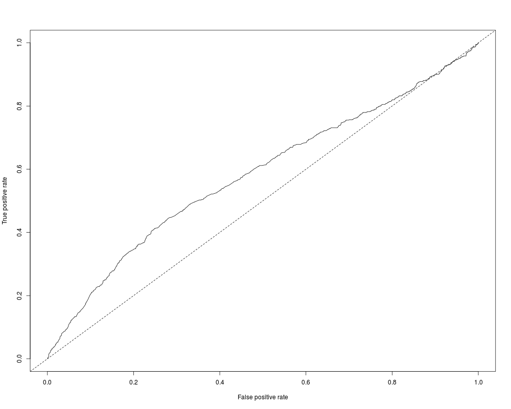
plot(performance(nokids_p3_pred, "tpr", "fpr"))
abline(0, 1, lty = 2)
performance(nokids_p3_pred, "auc")
plot(performance(nokids_l3_pred, "tpr", "fpr"))
abline(0, 1, lty = 2)
performance(nokids_l3_pred, "auc")@y.values
## Chapter 7
## Table 7.3
## subset selection
gss02 <- subset(GSS7402, year == 2002 & (age < 40 | !is.na(agefirstbirth)))
#Z# This selection conforms with top of page 229. However, there
#Z# are too many observations: 1374. Furthermore, there are six
#Z# observations with agefirstbirth <= 14 which will cause problems in
#Z# taking logs!
## computing time to first birth
gss02$tfb <- with(gss02, ifelse(is.na(agefirstbirth), age - 14, agefirstbirth - 14))
#Z# currently this is still needed before taking logs
gss02$tfb <- pmax(gss02$tfb, 1)
tfb_tobit <- tobit(log(tfb) ~ education + ethnicity + siblings + city16 + immigrant,
data = gss02, left = -Inf, right = log(gss02$age - 14))
tfb_ols <- lm(log(tfb) ~ education + ethnicity + siblings + city16 + immigrant,
data = gss02, subset = !is.na(agefirstbirth))
## Chapter 8
## Example 8.3
gss2002 <- subset(GSS7402, year == 2002 & (agefirstbirth < 40 | age < 40))
gss2002$afb <- with(gss2002, Surv(ifelse(kids > 0, agefirstbirth, age), kids > 0))
afb_km <- survfit(afb ~ 1, data = gss2002)
afb_skm <- summary(afb_km)
print(afb_skm)
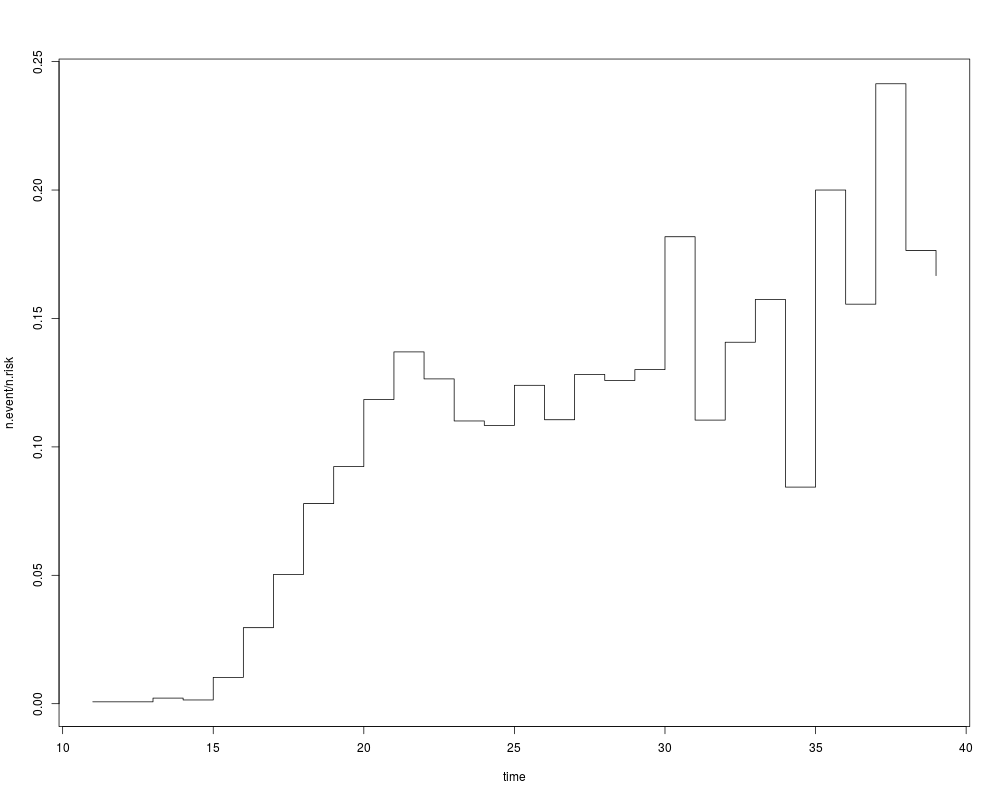
with(afb_skm, plot(n.event/n.risk ~ time, type = "s"))
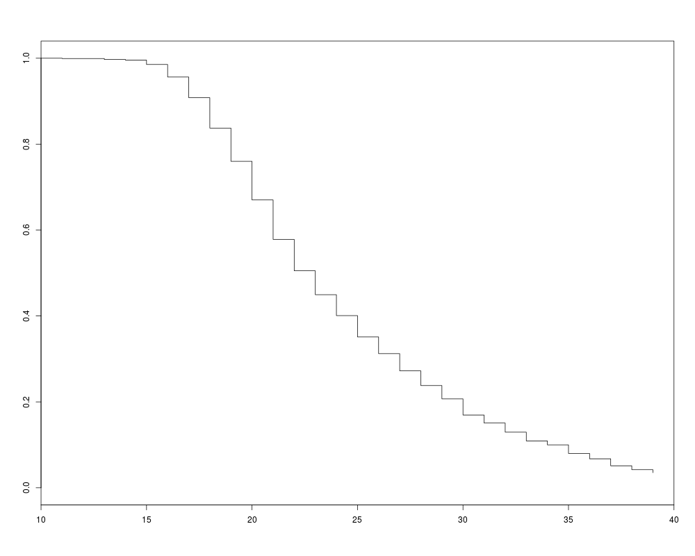
plot(afb_km, xlim = c(10, 40), conf.int = FALSE)
## Example 8.9
library("survival")
afb_ex <- survreg(
afb ~ education + siblings + ethnicity + immigrant + lowincome16 + city16,
data = gss2002, dist = "exponential")
afb_wb <- survreg(
afb ~ education + siblings + ethnicity + immigrant + lowincome16 + city16,
data = gss2002, dist = "weibull")
afb_ln <- survreg(
afb ~ education + siblings + ethnicity + immigrant + lowincome16 + city16,
data = gss2002, dist = "lognormal")
## Example 8.11
kids_pois <- glm(kids ~ education + trend + ethnicity + immigrant + lowincome16 + city16,
data = gss40, family = poisson)
library("MASS")
kids_nb <- glm.nb(kids ~ education + trend + ethnicity + immigrant + lowincome16 + city16,
data = gss40)
lrtest(kids_pois, kids_nb)
############################################
## German Socio-Economic Panel 1994--2002 ##
############################################
## data
data("GSOEP9402", package = "AER")
## some convenience data transformations
gsoep <- GSOEP9402
gsoep$meducation2 <- cut(gsoep$meducation, breaks = c(6, 10.25, 12.25, 18),
labels = c("7-10", "10.5-12", "12.5-18"))
gsoep$year2 <- factor(gsoep$year)
## Chapter 1
## Table 1.4 plus visualizations
gsoep_tab <- xtabs(~ meducation2 + school, data = gsoep)
round(prop.table(gsoep_tab, 1) * 100, digits = 2)
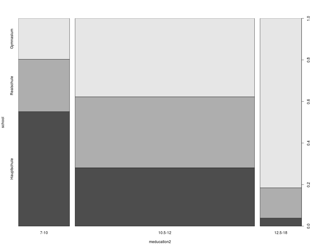
spineplot(gsoep_tab)
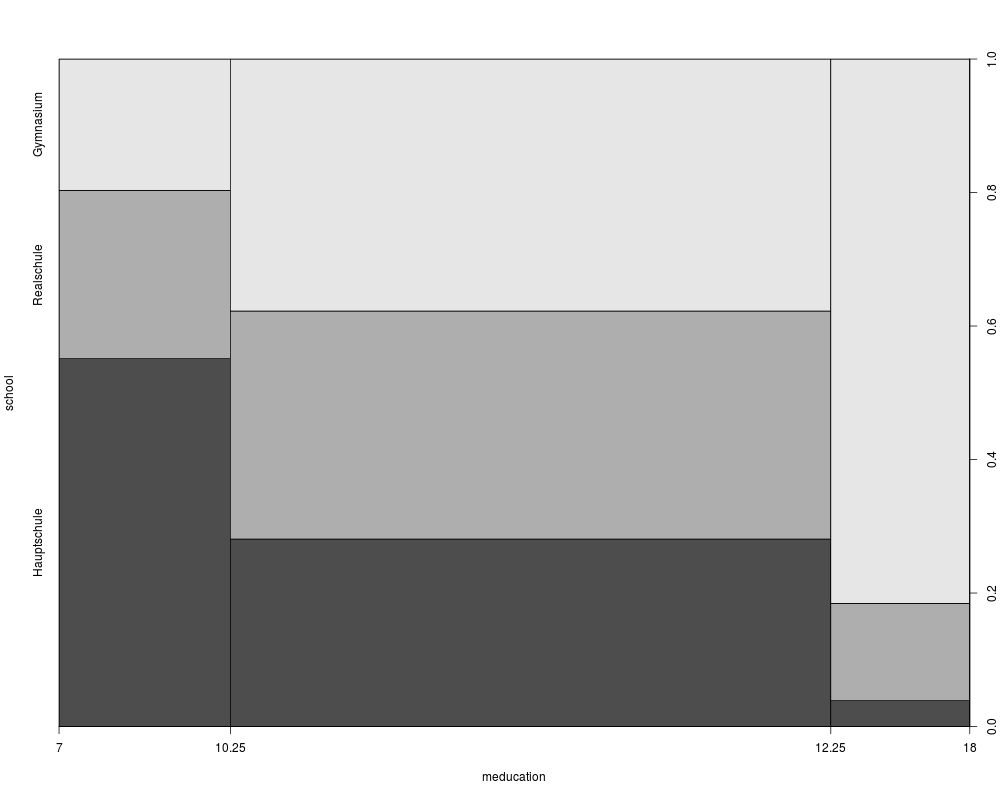
plot(school ~ meducation, data = gsoep, breaks = c(7, 10.25, 12.25, 18))
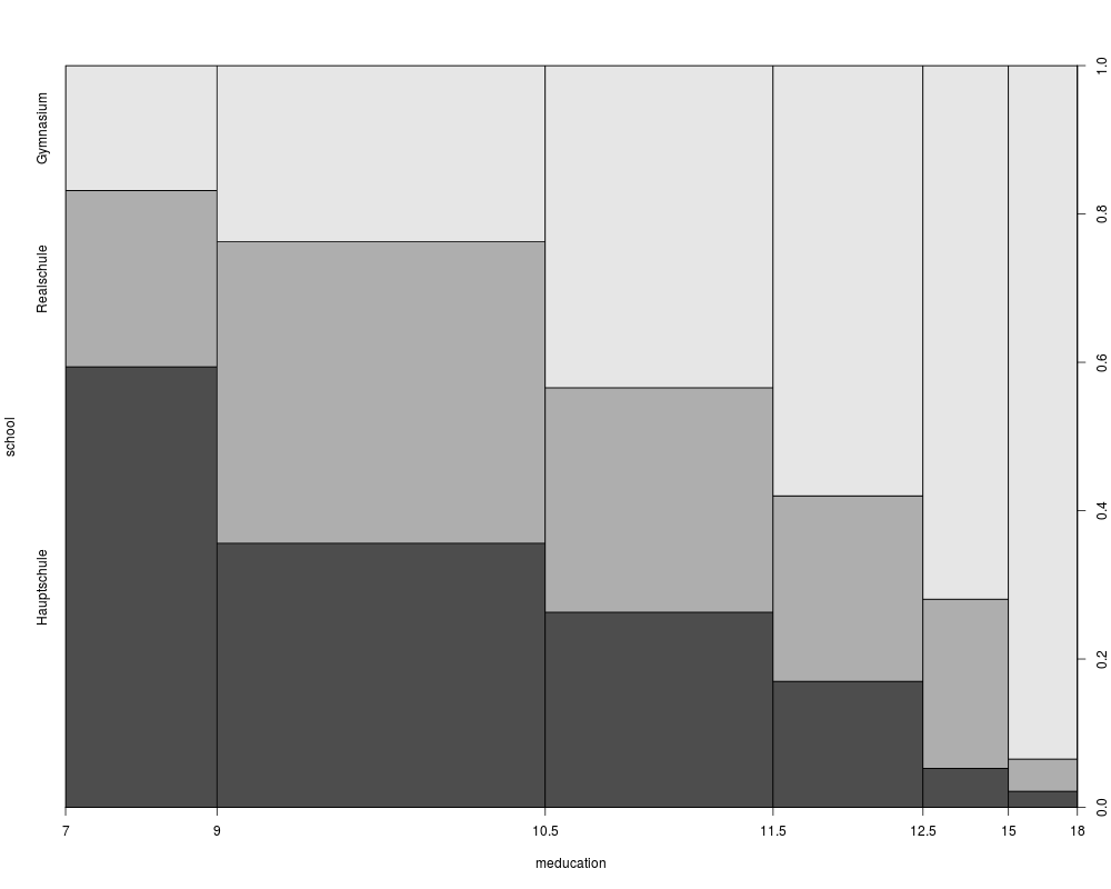
plot(school ~ meducation, data = gsoep, breaks = c(7, 9, 10.5, 11.5, 12.5, 15, 18))
## Chapter 5
## Table 5.1
library("nnet")
gsoep_mnl <- multinom(
school ~ meducation + memployment + log(income) + log(size) + parity + year2,
data = gsoep)
coeftest(gsoep_mnl)[c(1:6, 1:6 + 14),]
## alternatively
if(require("mlogit")) {
gsoep_mnl2 <- mlogit(school ~ 0 | meducation + memployment + log(income) +
log(size) + parity + year2, data = gsoep, shape = "wide", reflevel = "Hauptschule")
coeftest(gsoep_mnl2)[1:12,]
}
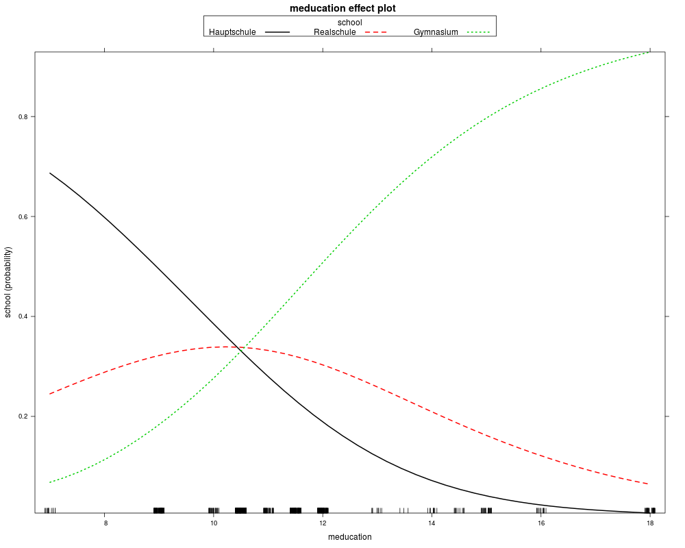
## Table 5.2
library("effects")
gsoep_eff <- effect("meducation", gsoep_mnl,
xlevels = list(meducation = sort(unique(gsoep$meducation))))
gsoep_eff$prob
plot(gsoep_eff, confint = FALSE)
## Table 5.3, odds
exp(coef(gsoep_mnl)[, "meducation"])
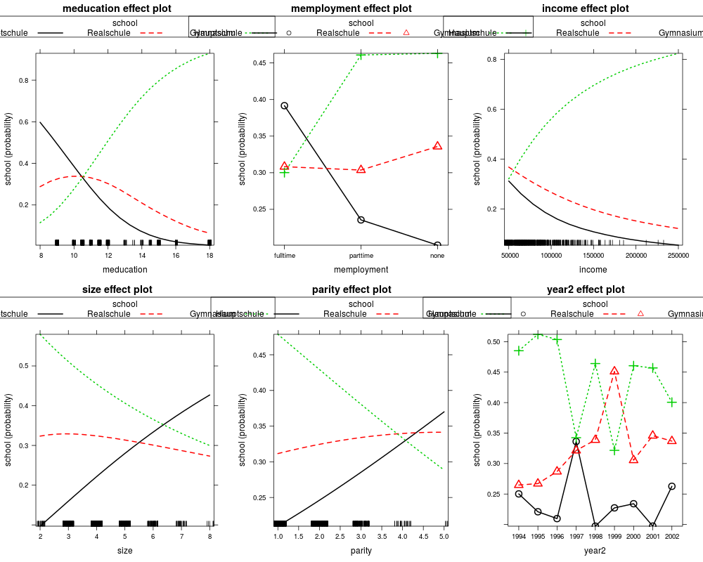
## all effects
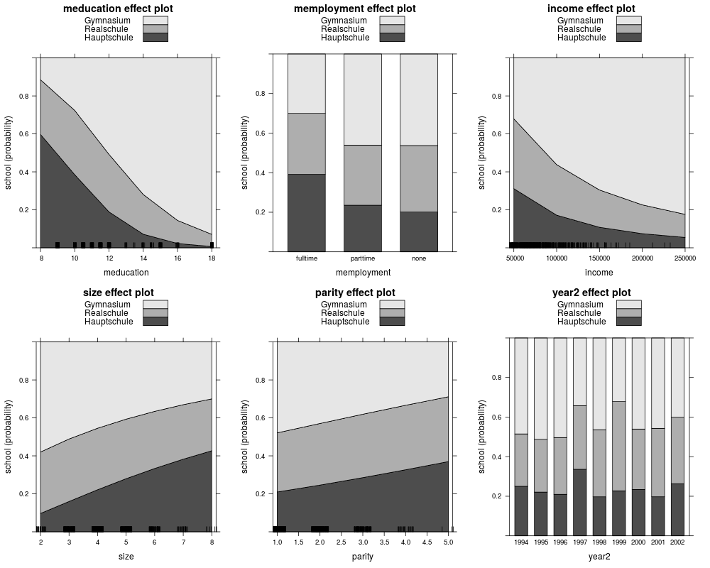
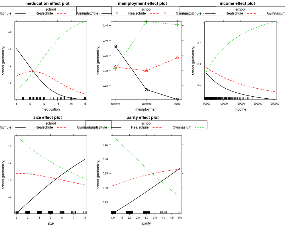
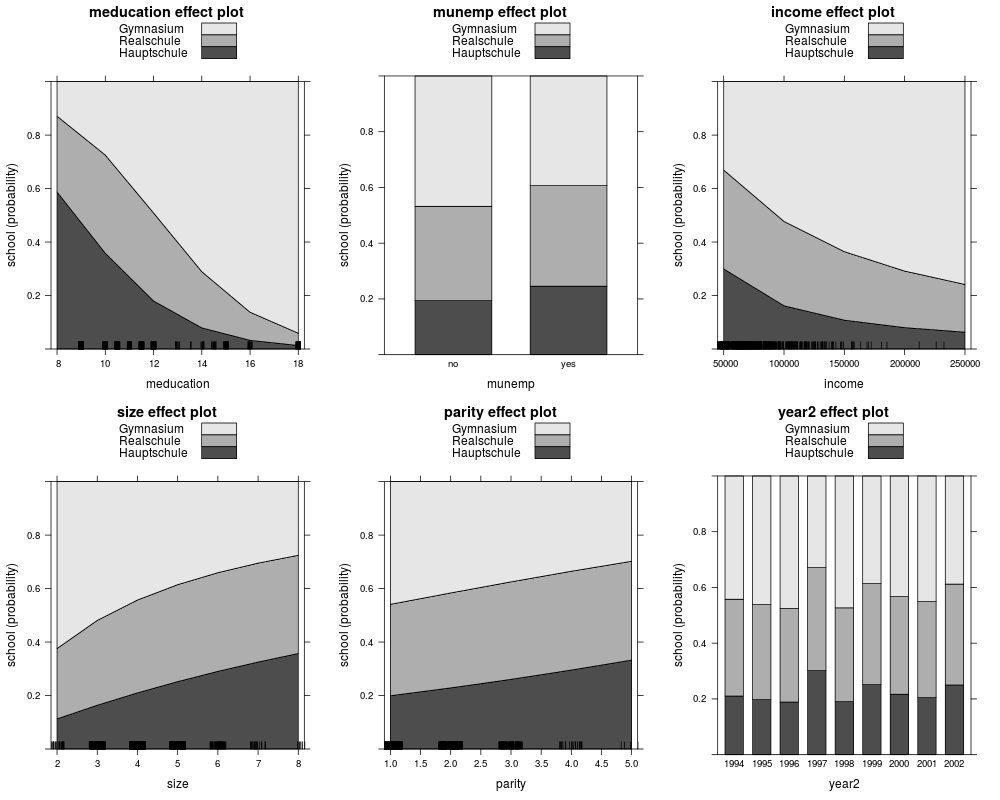
eff_mnl <- allEffects(gsoep_mnl)
plot(eff_mnl, ask = FALSE, confint = FALSE)
plot(eff_mnl, ask = FALSE, style = "stacked", colors = gray.colors(3))
## omit year
gsoep_mnl1 <- multinom(
school ~ meducation + memployment + log(income) + log(size) + parity,
data = gsoep)
lrtest(gsoep_mnl, gsoep_mnl1)
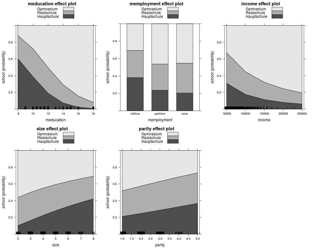
eff_mnl1 <- allEffects(gsoep_mnl1)
plot(eff_mnl1, ask = FALSE, confint = FALSE)
plot(eff_mnl1, ask = FALSE, style = "stacked", colors = gray.colors(3))
## Chapter 6
## Table 6.1
library("MASS")
gsoep$munemp <- factor(gsoep$memployment != "none",
levels = c(FALSE, TRUE), labels = c("no", "yes"))
gsoep_pop <- polr(school ~ meducation + munemp + log(income) + log(size) + parity + year2,
data = gsoep, method = "probit", Hess = TRUE)
gsoep_pol <- polr(school ~ meducation + munemp + log(income) + log(size) + parity + year2,
data = gsoep, Hess = TRUE)
lrtest(gsoep_pop)
lrtest(gsoep_pol)
## Table 6.2
## todo
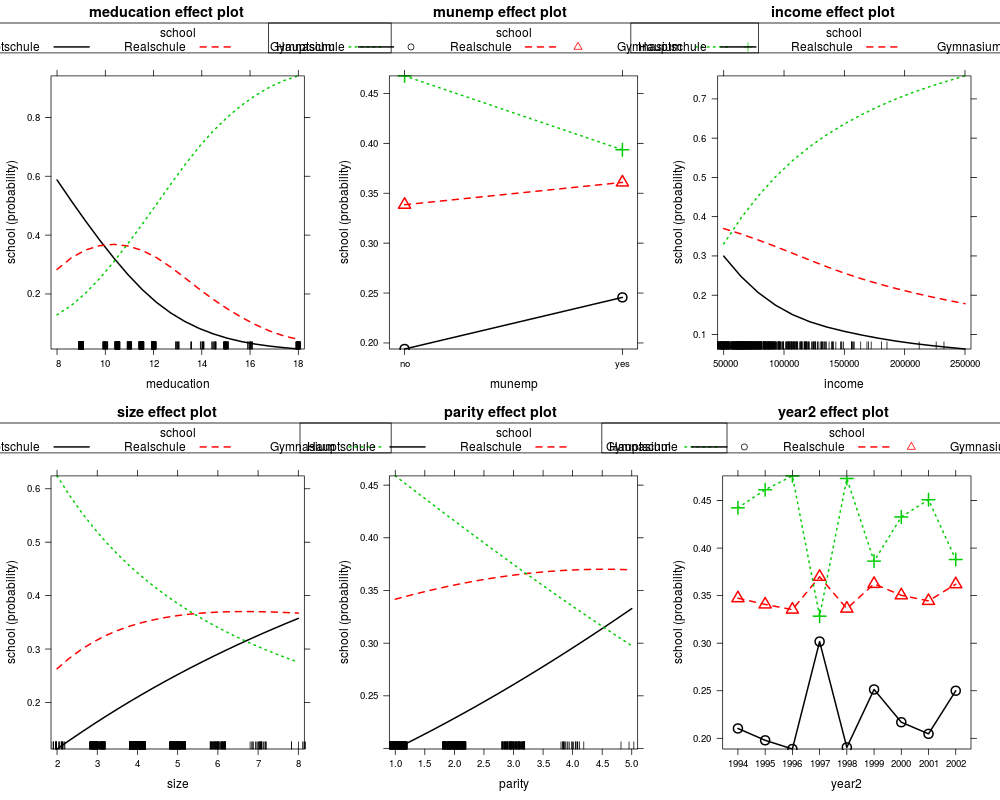
eff_pol <- allEffects(gsoep_pol)
plot(eff_pol, ask = FALSE, confint = FALSE)
plot(eff_pol, ask = FALSE, style = "stacked", colors = gray.colors(3))
####################################
## Labor Force Participation Data ##
####################################
## Mroz data
data("PSID1976", package = "AER")
PSID1976$nwincome <- with(PSID1976, (fincome - hours * wage)/1000)
## visualizations
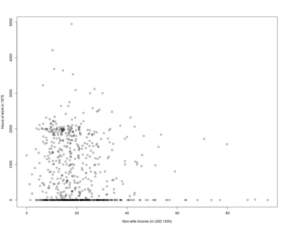
plot(hours ~ nwincome, data = PSID1976,
xlab = "Non-wife income (in USD 1000)",
ylab = "Hours of work in 1975")
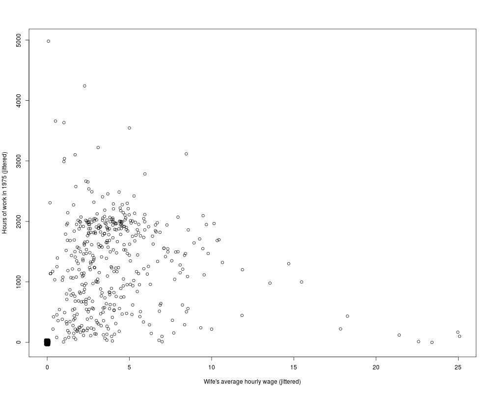
plot(jitter(hours, 200) ~ jitter(wage, 50), data = PSID1976,
xlab = "Wife's average hourly wage (jittered)",
ylab = "Hours of work in 1975 (jittered)")
## Chapter 1, p. 18
hours_lm <- lm(hours ~ wage + nwincome + youngkids + oldkids, data = PSID1976,
subset = participation == "yes")
## Chapter 7
## Example 7.2, Table 7.1
hours_tobit <- tobit(hours ~ nwincome + education + experience + I(experience^2) +
age + youngkids + oldkids, data = PSID1976)
hours_ols1 <- lm(hours ~ nwincome + education + experience + I(experience^2) +
age + youngkids + oldkids, data = PSID1976)
hours_ols2 <- lm(hours ~ nwincome + education + experience + I(experience^2) +
age + youngkids + oldkids, data = PSID1976, subset = participation == "yes")
## Example 7.10, Table 7.4
wage_ols <- lm(log(wage) ~ education + experience + I(experience^2),
data = PSID1976, subset = participation == "yes")
library("sampleSelection")
wage_ghr <- selection(participation ~ nwincome + age + youngkids + oldkids +
education + experience + I(experience^2),
log(wage) ~ education + experience + I(experience^2), data = PSID1976)
## Exercise 7.13
hours_cragg1 <- glm(participation ~ nwincome + education +
experience + I(experience^2) + age + youngkids + oldkids,
data = PSID1976, family = binomial(link = "probit"))
library("truncreg")
hours_cragg2 <- truncreg(hours ~ nwincome + education +
experience + I(experience^2) + age + youngkids + oldkids,
data = PSID1976, subset = participation == "yes")
## Exercise 7.15
wage_olscoef <- sapply(c(-Inf, 0.5, 1, 1.5, 2), function(censpoint)
coef(lm(log(wage) ~ education + experience + I(experience^2),
data = PSID1976[log(PSID1976$wage) > censpoint,])))
wage_mlcoef <- sapply(c(0.5, 1, 1.5, 2), function(censpoint)
coef(tobit(log(wage) ~ education + experience + I(experience^2),
data = PSID1976, left = censpoint)))
##################################
## Choice of Brand for Crackers ##
##################################
## data
if(require("mlogit")) {
data("Cracker", package = "mlogit")
head(Cracker, 3)
crack <- mlogit.data(Cracker, varying = 2:13, shape = "wide", choice = "choice")
head(crack, 12)
## Table 5.6 (model 3 probably not fully converged in W&B)
crack$price <- crack$price/100
crack_mlogit1 <- mlogit(choice ~ price | 0, data = crack, reflevel = "private")
crack_mlogit2 <- mlogit(choice ~ price | 1, data = crack, reflevel = "private")
crack_mlogit3 <- mlogit(choice ~ price + feat + disp | 1, data = crack,
reflevel = "private")
lrtest(crack_mlogit1, crack_mlogit2, crack_mlogit3)
## IIA test
crack_mlogit_all <- update(crack_mlogit2, reflevel = "nabisco")
crack_mlogit_res <- update(crack_mlogit_all,
alt.subset = c("keebler", "nabisco", "sunshine"))
hmftest(crack_mlogit_all, crack_mlogit_res)
}
Results
R version 3.3.1 (2016-06-21) -- "Bug in Your Hair"
Copyright (C) 2016 The R Foundation for Statistical Computing
Platform: x86_64-pc-linux-gnu (64-bit)

R is free software and comes with ABSOLUTELY NO WARRANTY.
You are welcome to redistribute it under certain conditions.
Type 'license()' or 'licence()' for distribution details.

R is a collaborative project with many contributors.
Type 'contributors()' for more information and
'citation()' on how to cite R or R packages in publications.

Type 'demo()' for some demos, 'help()' for on-line help, or
'help.start()' for an HTML browser interface to help.
Type 'q()' to quit R.

> library(AER)
Loading required package: car
Loading required package: lmtest
Loading required package: zoo

Attaching package: 'zoo'

The following objects are masked from 'package:base':

    as.Date, as.Date.numeric

Loading required package: sandwich
Loading required package: survival
> png(filename="/home/ddbj/snapshot/RGM3/R_CC/result/AER/WinkelmannBoes2009.Rd_%03d_medium.png", width=480, height=480)
> ### Name: WinkelmannBoes2009
> ### Title: Data and Examples from Winkelmann and Boes (2009)
> ### Aliases: WinkelmannBoes2009
> ### Keywords: datasets
>
> ### ** Examples
>
> #########################################
> ## US General Social Survey 1974--2002 ##
> #########################################
>
> ## data
> data("GSS7402", package = "AER")
>
> ## completed fertility subset
> gss40 <- subset(GSS7402, age >= 40)
>
>
> ## Chapter 1
> ## Table 1.1
> gss_kids <- table(gss40$kids)
> cbind(absolute = gss_kids,
+   relative = round(prop.table(gss_kids) * 100, digits = 2))
  absolute relative
0      744    14.45
1      706    13.71
2     1368    26.56
3     1002    19.46
4      593    11.51
5      309     6.00
6      190     3.69
7       89     1.73
8      149     2.89
>
> ## Table 1.2
> sd1 <- function(x) sd(x) / sqrt(length(x))
> with(gss40, round(cbind(
+   "obs"            = tapply(kids, year, length),
+   "av kids"        = tapply(kids, year, mean),
+   " " =              tapply(kids, year, sd1),
+   "prop childless" = tapply(kids, year, function(x) mean(x <= 0)),
+    " " =             tapply(kids, year, function(x) sd1(x <= 0)),
+   "av schooling"   = tapply(education, year, mean),
+    " " =             tapply(education, year, sd1)
+ ), digits = 2))
     obs av kids      prop childless      av schooling
1974 410    3.17 0.10           0.09 0.01        11.07 0.16
1978 445    2.73 0.09           0.14 0.02        11.00 0.15
1982 577    2.96 0.09           0.14 0.01        11.05 0.14
1986 470    2.70 0.09           0.16 0.02        11.34 0.14
1990 431    2.50 0.08           0.15 0.02        12.41 0.15
1994 989    2.40 0.06           0.15 0.01        12.78 0.10
1998 911    2.42 0.06           0.15 0.01        12.94 0.11
2002 917    2.36 0.06           0.16 0.01        13.25 0.10
>
> ## Table 1.3
> gss40$trend <- gss40$year - 1974
> kids_lm1 <- lm(kids ~ factor(year), data = gss40)
> kids_lm2 <- lm(kids ~ trend, data = gss40)
> kids_lm3 <- lm(kids ~ trend + education, data = gss40)
>
>
> ## Chapter 2
> ## Table 2.1
> kids_tab <- prop.table(xtabs(~ kids + year, data = gss40), 2) * 100
> round(kids_tab[,c(4, 8)], digits = 2)
    year
kids  1986  2002
   0 16.38 15.59
   1 11.28 13.96
   2 26.60 28.68
   3 15.74 22.14
   4 11.49  9.92
   5  7.02  3.93
   6  6.38  2.62
   7  1.70  1.64
   8  3.40  1.53
> ## Figure 2.1
> barplot(t(kids_tab[, c(4, 8)]), beside = TRUE, legend = TRUE)
>
>
> ## Chapter 3, Example 3.14
> ## Table 3.1
> gss40$nokids <- factor(gss40$kids <= 0,
+   levels = c(FALSE, TRUE), labels = c("no", "yes"))
> nokids_p1 <- glm(nokids ~ 1, data = gss40, family = binomial(link = "probit"))
> nokids_p2 <- glm(nokids ~ trend, data = gss40, family = binomial(link = "probit"))
> nokids_p3 <- glm(nokids ~ trend + education + ethnicity + siblings,
+   data = gss40, family = binomial(link = "probit"))
>
> ## p. 87
> lrtest(nokids_p1, nokids_p2, nokids_p3)
Likelihood ratio test

Model 1: nokids ~ 1
Model 2: nokids ~ trend
Model 3: nokids ~ trend + education + ethnicity + siblings
  #Df  LogLik Df   Chisq Pr(>Chisq)
1   1 -2126.9
2   2 -2123.6  1  6.5677    0.01038 *
3   5 -2107.1  3 32.9906  3.235e-07 ***
---
Signif. codes:  0 '***' 0.001 '**' 0.01 '*' 0.05 '.' 0.1 ' ' 1
>
> ## Chapter 4, Example 4.1
> gss40$nokids01 <- as.numeric(gss40$nokids) - 1
> nokids_lm3 <- lm(nokids01 ~ trend + education + ethnicity + siblings, data = gss40)
> coeftest(nokids_lm3, vcov = sandwich)

t test of coefficients:

                 Estimate  Std. Error t value  Pr(>|t|)
(Intercept)    0.03972864  0.02898580  1.3706    0.1706
trend          0.00060242  0.00053829  1.1191    0.2631
education      0.00757341  0.00187637  4.0362 5.511e-05 ***
ethnicitycauc  0.01424775  0.01314836  1.0836    0.2786
siblings      -0.00235388  0.00153770 -1.5308    0.1259
---
Signif. codes:  0 '***' 0.001 '**' 0.01 '*' 0.05 '.' 0.1 ' ' 1

>
> ## Example 4.3
> ## Table 4.1
> nokids_l1 <- glm(nokids ~ 1, data = gss40, family = binomial(link = "logit"))
> nokids_l3 <- glm(nokids ~ trend + education + ethnicity + siblings,
+   data = gss40, family = binomial(link = "logit"))
> lrtest(nokids_p3)
Likelihood ratio test

Model 1: nokids ~ trend + education + ethnicity + siblings
Model 2: nokids ~ 1
  #Df  LogLik Df  Chisq Pr(>Chisq)
1   5 -2107.1
2   1 -2126.9 -4 39.558  5.341e-08 ***
---
Signif. codes:  0 '***' 0.001 '**' 0.01 '*' 0.05 '.' 0.1 ' ' 1
> lrtest(nokids_l3)
Likelihood ratio test

Model 1: nokids ~ trend + education + ethnicity + siblings
Model 2: nokids ~ 1
  #Df  LogLik Df  Chisq Pr(>Chisq)
1   5 -2106.0
2   1 -2126.9 -4 41.859  1.784e-08 ***
---
Signif. codes:  0 '***' 0.001 '**' 0.01 '*' 0.05 '.' 0.1 ' ' 1
>
> ## Table 4.2
> nokids_xbar <- colMeans(model.matrix(nokids_l3))
> sum(coef(nokids_p3) * nokids_xbar)
[1] -1.069858
> sum(coef(nokids_l3) * nokids_xbar)
[1] -1.802965
> dnorm(sum(coef(nokids_p3) * nokids_xbar))
[1] 0.2250941
> dlogis(sum(coef(nokids_l3) * nokids_xbar))
[1] 0.1214709
> dnorm(sum(coef(nokids_p3) * nokids_xbar)) * coef(nokids_p3)[3]
  education
0.007072723
> dlogis(sum(coef(nokids_l3) * nokids_xbar)) * coef(nokids_l3)[3]
  education
0.007658209
> exp(coef(nokids_l3)[3])
education
 1.065075
>
> ## Figure 4.4
> ## everything by hand (for ethnicity = "cauc" group)
> nokids_xbar <- as.vector(nokids_xbar)
> nokids_nd <- data.frame(education = seq(0, 20, by = 0.5), trend = nokids_xbar[2],
+   ethnicity = "cauc", siblings = nokids_xbar[4])
> nokids_p3_fit <- predict(nokids_p3, newdata = nokids_nd,
+   type = "response", se.fit = TRUE)
> plot(nokids_nd$education, nokids_p3_fit$fit, type = "l",
+   xlab = "education", ylab = "predicted probability", ylim = c(0, 0.3))
> polygon(c(nokids_nd$education, rev(nokids_nd$education)),
+   c(nokids_p3_fit$fit + 1.96 * nokids_p3_fit$se.fit,
+   rev(nokids_p3_fit$fit - 1.96 * nokids_p3_fit$se.fit)),
+   col = "lightgray", border = "lightgray")
> lines(nokids_nd$education, nokids_p3_fit$fit)
>
> ## using "effects" package (for average "ethnicity" variable)
> library("effects")

Attaching package: 'effects'

The following object is masked from 'package:car':

    Prestige

> nokids_p3_ef <- effect("education", nokids_p3, xlevels = list(education = 0:20))
> plot(nokids_p3_ef, rescale.axis = FALSE, ylim = c(0, 0.3))
NOTE: the rescale.axis argument is deprecated; use type instead
>
> ## using "effects" plus modification by hand
> nokids_p3_ef1 <- as.data.frame(nokids_p3_ef)
> plot(pnorm(fit) ~ education, data = nokids_p3_ef1, type = "n", ylim = c(0, 0.3))
> polygon(c(0:20, 20:0), pnorm(c(nokids_p3_ef1$upper, rev(nokids_p3_ef1$lower))),
+   col = "lightgray", border = "lightgray")
> lines(pnorm(fit) ~ education, data = nokids_p3_ef1)
>
> ## Table 4.6
> ## McFadden's R^2
> 1 - as.numeric( logLik(nokids_p3) / logLik(nokids_p1) )
[1] 0.009299554
> 1 - as.numeric( logLik(nokids_l3) / logLik(nokids_l1) )
[1] 0.009840523
> ## McKelvey and Zavoina R^2
> r2mz <- function(obj) {
+   ystar <- predict(obj)
+   sse <- sum((ystar - mean(ystar))^2)
+   s2 <- switch(obj$family$link, "probit" = 1, "logit" = pi^2/3, NA)
+   n <- length(residuals(obj))
+   sse / (n * s2 + sse)
+ }
> r2mz(nokids_p3)
[1] 0.01784602
> r2mz(nokids_l3)
[1] 0.02076783
> ## AUC
> library("ROCR")
Loading required package: gplots

Attaching package: 'gplots'

The following object is masked from 'package:stats':

    lowess

> nokids_p3_pred <- prediction(fitted(nokids_p3), gss40$nokids)
> nokids_l3_pred <- prediction(fitted(nokids_l3), gss40$nokids)
> plot(performance(nokids_p3_pred, "tpr", "fpr"))
> abline(0, 1, lty = 2)
> performance(nokids_p3_pred, "auc")
An object of class "performance"
Slot "x.name":
[1] "None"

Slot "y.name":
[1] "Area under the ROC curve"

Slot "alpha.name":
[1] "none"

Slot "x.values":
list()

Slot "y.values":
[[1]]
[1] 0.5828144


Slot "alpha.values":
list()

> plot(performance(nokids_l3_pred, "tpr", "fpr"))
> abline(0, 1, lty = 2)
> performance(nokids_l3_pred, "auc")@y.values
[[1]]
[1] 0.5828855

>
> ## Chapter 7
> ## Table 7.3
> ## subset selection
> gss02 <- subset(GSS7402, year == 2002 & (age < 40 | !is.na(agefirstbirth)))
> #Z# This selection conforms with top of page 229. However, there
> #Z# are too many observations: 1374. Furthermore, there are six
> #Z# observations with agefirstbirth <= 14 which will cause problems in
> #Z# taking logs!
>
> ## computing time to first birth
> gss02$tfb <- with(gss02, ifelse(is.na(agefirstbirth), age - 14, agefirstbirth - 14))
> #Z# currently this is still needed before taking logs
> gss02$tfb <- pmax(gss02$tfb, 1)
>
> tfb_tobit <- tobit(log(tfb) ~ education + ethnicity + siblings + city16 + immigrant,
+   data = gss02, left = -Inf, right = log(gss02$age - 14))
> tfb_ols <- lm(log(tfb) ~ education + ethnicity + siblings + city16 + immigrant,
+   data = gss02, subset = !is.na(agefirstbirth))
>
> ## Chapter 8
> ## Example 8.3
> gss2002 <- subset(GSS7402, year == 2002 & (agefirstbirth < 40 | age < 40))
> gss2002$afb <- with(gss2002, Surv(ifelse(kids > 0, agefirstbirth, age), kids > 0))
> afb_km <- survfit(afb ~ 1, data = gss2002)
> afb_skm <- summary(afb_km)
> print(afb_skm)
Call: survfit(formula = afb ~ 1, data = gss2002)

 time n.risk n.event survival  std.err lower 95% CI upper 95% CI
   11   1371       1   0.9993 0.000729       0.9978       1.0000
   13   1370       3   0.9971 0.001457       0.9942       0.9999
   14   1367       2   0.9956 0.001783       0.9921       0.9991
   15   1365      14   0.9854 0.003238       0.9791       0.9918
   16   1351      40   0.9562 0.005525       0.9455       0.9671
   17   1311      66   0.9081 0.007802       0.8929       0.9235
   18   1245      97   0.8373 0.009967       0.8180       0.8571
   19   1148     106   0.7600 0.011534       0.7378       0.7830
   20   1030     122   0.6700 0.012726       0.6455       0.6954
   21    898     123   0.5782 0.013406       0.5525       0.6051
   22    767      97   0.5051 0.013612       0.4791       0.5325
   23    654      72   0.4495 0.013600       0.4236       0.4770
   24    563      61   0.4008 0.013480       0.3752       0.4281
   25    484      60   0.3511 0.013248       0.3261       0.3781
   26    407      45   0.3123 0.012986       0.2878       0.3388
   27    351      45   0.2723 0.012618       0.2486       0.2981
   28    294      37   0.2380 0.012223       0.2152       0.2632
   29    246      32   0.2070 0.011795       0.1852       0.2315
   30    209      38   0.1694 0.011119       0.1489       0.1926
   31    163      18   0.1507 0.010730       0.1311       0.1733
   32    135      19   0.1295 0.010264       0.1108       0.1512
   33    108      17   0.1091 0.009766       0.0915       0.1300
   34     83       7   0.0999 0.009542       0.0828       0.1205
   35     65      13   0.0799 0.009101       0.0639       0.0999
   36     45       7   0.0675 0.008815       0.0522       0.0872
   37     29       7   0.0512 0.008572       0.0369       0.0711
   38     17       3   0.0422 0.008499       0.0284       0.0626
   39     12       2   0.0351 0.008411       0.0220       0.0562
> with(afb_skm, plot(n.event/n.risk ~ time, type = "s"))
> plot(afb_km, xlim = c(10, 40), conf.int = FALSE)
>
> ## Example 8.9
> library("survival")
> afb_ex <- survreg(
+   afb ~ education + siblings + ethnicity + immigrant + lowincome16 + city16,
+   data = gss2002, dist = "exponential")
> afb_wb <- survreg(
+   afb ~ education + siblings + ethnicity + immigrant + lowincome16 + city16,
+   data = gss2002, dist = "weibull")
> afb_ln <- survreg(
+   afb ~ education + siblings + ethnicity + immigrant + lowincome16 + city16,
+   data = gss2002, dist = "lognormal")
>
> ## Example 8.11
> kids_pois <- glm(kids ~ education + trend + ethnicity + immigrant + lowincome16 + city16,
+   data = gss40, family = poisson)
> library("MASS")
> kids_nb <- glm.nb(kids ~ education + trend + ethnicity + immigrant + lowincome16 + city16,
+   data = gss40)
> lrtest(kids_pois, kids_nb)
Likelihood ratio test

Model 1: kids ~ education + trend + ethnicity + immigrant + lowincome16 +
    city16
Model 2: kids ~ education + trend + ethnicity + immigrant + lowincome16 +
    city16
  #Df LogLik Df  Chisq Pr(>Chisq)
1   7 -10117
2   8 -10014  1 205.17  < 2.2e-16 ***
---
Signif. codes:  0 '***' 0.001 '**' 0.01 '*' 0.05 '.' 0.1 ' ' 1
>
>
> ############################################
> ## German Socio-Economic Panel 1994--2002 ##
> ############################################
>
> ## data
> data("GSOEP9402", package = "AER")
>
> ## some convenience data transformations
> gsoep <- GSOEP9402
> gsoep$meducation2 <- cut(gsoep$meducation, breaks = c(6, 10.25, 12.25, 18),
+   labels = c("7-10", "10.5-12", "12.5-18"))
> gsoep$year2 <- factor(gsoep$year)
>
> ## Chapter 1
> ## Table 1.4 plus visualizations
> gsoep_tab <- xtabs(~ meducation2 + school, data = gsoep)
> round(prop.table(gsoep_tab, 1) * 100, digits = 2)
           school
meducation2 Hauptschule Realschule Gymnasium
    7-10          55.12      25.20     19.69
    10.5-12       28.09      34.16     37.75
    12.5-18        3.88      14.56     81.55
> spineplot(gsoep_tab)
> plot(school ~ meducation, data = gsoep, breaks = c(7, 10.25, 12.25, 18))
> plot(school ~ meducation, data = gsoep, breaks = c(7, 9, 10.5, 11.5, 12.5, 15, 18))
>
>
> ## Chapter 5
> ## Table 5.1
> library("nnet")
> gsoep_mnl <- multinom(
+   school ~ meducation + memployment + log(income) + log(size) + parity + year2,
+   data = gsoep)
# weights:  48 (30 variable)
initial  value 741.563295
iter  10 value 655.748279
iter  20 value 624.992858
iter  30 value 618.605354
final  value 618.475696
converged
> coeftest(gsoep_mnl)[c(1:6, 1:6 + 14),]
                                  Estimate Std. Error    z value     Pr(>|z|)
Realschule:(Intercept)          -6.3864877 2.36903996 -2.6958126 7.021716e-03
Realschule:meducation            0.3004843 0.07910641  3.7984819 1.455851e-04
Realschule:memploymentparttime   0.4933680 0.32189721  1.5326879 1.253528e-01
Realschule:memploymentnone       0.7526399 0.32884476  2.2887392 2.209451e-02
Realschule:log(income)           0.3934871 0.22539836  1.7457408 8.085601e-02
Realschule:log(size)            -1.1921790 0.44641156 -2.6705827 7.571972e-03
Realschule:year22002             0.1922413 0.45158350  0.4257049 6.703229e-01
Gymnasium:(Intercept)          -23.6975758 3.01022807 -7.8723523 3.480345e-15
Gymnasium:meducation             0.6597649 0.08144034  8.1012060 5.441700e-16
Gymnasium:memploymentparttime    0.9372429 0.34536421  2.7137813 6.652007e-03
Gymnasium:memploymentnone        1.1007579 0.35842760  3.0710746 2.132898e-03
Gymnasium:log(income)            1.6676745 0.28408439  5.8703492 4.348783e-09
>
> ## alternatively
> if(require("mlogit")) {
+ gsoep_mnl2 <- mlogit(school ~ 0 | meducation + memployment + log(income) +
+   log(size) + parity + year2, data = gsoep, shape = "wide", reflevel = "Hauptschule")
+ coeftest(gsoep_mnl2)[1:12,]
+ }
Loading required package: mlogit
Loading required package: Formula
Loading required package: maxLik
Loading required package: miscTools

Please cite the 'maxLik' package as:
Henningsen, Arne and Toomet, Ott (2011). maxLik: A package for maximum likelihood estimation in R. Computational Statistics 26(3), 443-458. DOI 10.1007/s00180-010-0217-1.

If you have questions, suggestions, or comments regarding the 'maxLik' package, please use a forum or 'tracker' at maxLik's R-Forge site:
https://r-forge.r-project.org/projects/maxlik/
                                  Estimate Std. Error   t value     Pr(>|t|)
Gymnasium:(intercept)          -23.6982768 3.01026604 -7.872486 1.475202e-14
Realschule:(intercept)          -6.3865987 2.36904833 -2.695850 7.204061e-03
Gymnasium:meducation             0.6597829 0.08144157  8.101304 2.726719e-15
Realschule:meducation            0.3004923 0.07910725  3.798543 1.593085e-04
Gymnasium:memploymentparttime    0.9372401 0.34536576  2.713761 6.830145e-03
Realschule:memploymentparttime   0.4933644 0.32189760  1.532675 1.258463e-01
Gymnasium:memploymentnone        1.1007670 0.35842942  3.071084 2.222541e-03
Realschule:memploymentnone       0.7526490 0.32884523  2.288764 2.241551e-02
Gymnasium:log(income)            1.6677258 0.28408738  5.870468 6.954975e-09
Realschule:log(income)           0.3934899 0.22539876  1.745750 8.133056e-02
Gymnasium:log(size)             -1.5459256 0.48775919 -3.169444 1.599570e-03
Realschule:log(size)            -1.1921835 0.44641174 -2.670592 7.762668e-03
>
> ## Table 5.2
> library("effects")
> gsoep_eff <- effect("meducation", gsoep_mnl,
+   xlevels = list(meducation = sort(unique(gsoep$meducation))))
> gsoep_eff$prob
      prob.Hauptschule prob.Realschule prob.Gymnasium
 [1,]      0.686724467      0.24514452     0.06813102
 [2,]      0.494486442      0.32195219     0.18356137
 [3,]      0.385007121      0.33853566     0.27645721
 [4,]      0.331068546      0.33830072     0.33063074
 [5,]      0.279605513      0.33203209     0.38836239
 [6,]      0.231922018      0.32005576     0.44802222
 [7,]      0.189019319      0.30313717     0.50784351
 [8,]      0.119575666      0.25898492     0.62143941
 [9,]      0.093066080      0.23424613     0.67268779
[10,]      0.071541719      0.20926168     0.71919660
[11,]      0.054404764      0.18493393     0.76066131
[12,]      0.040990572      0.16192466     0.79708477
[13,]      0.022753542      0.12138826     0.85585820
[14,]      0.006601958      0.06423885     0.92915919
> plot(gsoep_eff, confint = FALSE)
>
> ## Table 5.3, odds
> exp(coef(gsoep_mnl)[, "meducation"])
Realschule  Gymnasium
  1.350513   1.934338
>
> ## all effects
> eff_mnl <- allEffects(gsoep_mnl)
> plot(eff_mnl, ask = FALSE, confint = FALSE)
> plot(eff_mnl, ask = FALSE, style = "stacked", colors = gray.colors(3))
>
> ## omit year
> gsoep_mnl1 <- multinom(
+   school ~ meducation + memployment + log(income) + log(size) + parity,
+   data = gsoep)
# weights:  24 (14 variable)
initial  value 741.563295
iter  10 value 658.442291
iter  20 value 624.980518
final  value 624.957624
converged
> lrtest(gsoep_mnl, gsoep_mnl1)
Likelihood ratio test

Model 1: school ~ meducation + memployment + log(income) + log(size) +
    parity + year2
Model 2: school ~ meducation + memployment + log(income) + log(size) +
    parity
  #Df  LogLik  Df  Chisq Pr(>Chisq)
1  30 -618.48
2  14 -624.96 -16 12.964     0.6754
> eff_mnl1 <- allEffects(gsoep_mnl1)
> plot(eff_mnl1, ask = FALSE, confint = FALSE)
> plot(eff_mnl1, ask = FALSE, style = "stacked", colors = gray.colors(3))
>
>
> ## Chapter 6
> ## Table 6.1
> library("MASS")
> gsoep$munemp <- factor(gsoep$memployment != "none",
+   levels = c(FALSE, TRUE), labels = c("no", "yes"))
> gsoep_pop <- polr(school ~ meducation + munemp + log(income) + log(size) + parity + year2,
+   data = gsoep, method = "probit", Hess = TRUE)
> gsoep_pol <- polr(school ~ meducation + munemp + log(income) + log(size) + parity + year2,
+   data = gsoep, Hess = TRUE)
> lrtest(gsoep_pop)
Likelihood ratio test

Model 1: school ~ meducation + munemp + log(income) + log(size) + parity +
    year2
Model 2: school ~ 1
  #Df  LogLik  Df  Chisq Pr(>Chisq)
1  15 -631.19
2   2 -732.84 -13 203.31  < 2.2e-16 ***
---
Signif. codes:  0 '***' 0.001 '**' 0.01 '*' 0.05 '.' 0.1 ' ' 1
> lrtest(gsoep_pol)
Likelihood ratio test

Model 1: school ~ meducation + munemp + log(income) + log(size) + parity +
    year2
Model 2: school ~ 1
  #Df  LogLik  Df  Chisq Pr(>Chisq)
1  15 -630.15
2   2 -732.84 -13 205.38  < 2.2e-16 ***
---
Signif. codes:  0 '***' 0.001 '**' 0.01 '*' 0.05 '.' 0.1 ' ' 1
>
> ## Table 6.2
> ## todo
> eff_pol <- allEffects(gsoep_pol)
> plot(eff_pol, ask = FALSE, confint = FALSE)
> plot(eff_pol, ask = FALSE, style = "stacked", colors = gray.colors(3))
>
>
> ####################################
> ## Labor Force Participation Data ##
> ####################################
>
> ## Mroz data
> data("PSID1976", package = "AER")
> PSID1976$nwincome <- with(PSID1976, (fincome - hours * wage)/1000)
>
> ## visualizations
> plot(hours ~ nwincome, data = PSID1976,
+   xlab = "Non-wife income (in USD 1000)",
+   ylab = "Hours of work in 1975")
>
> plot(jitter(hours, 200) ~ jitter(wage, 50), data = PSID1976,
+   xlab = "Wife's average hourly wage (jittered)",
+   ylab = "Hours of work in 1975 (jittered)")
>
> ## Chapter 1, p. 18
> hours_lm <- lm(hours ~ wage + nwincome + youngkids + oldkids, data = PSID1976,
+   subset = participation == "yes")
>
> ## Chapter 7
> ## Example 7.2, Table 7.1
> hours_tobit <- tobit(hours ~ nwincome + education + experience + I(experience^2) +
+   age + youngkids + oldkids, data = PSID1976)
> hours_ols1 <- lm(hours ~ nwincome + education + experience + I(experience^2) +
+   age + youngkids + oldkids, data = PSID1976)
> hours_ols2 <- lm(hours ~ nwincome + education + experience + I(experience^2) +
+   age + youngkids + oldkids, data = PSID1976, subset = participation == "yes")
>
> ## Example 7.10, Table 7.4
> wage_ols <- lm(log(wage) ~ education + experience + I(experience^2),
+   data = PSID1976, subset = participation == "yes")
>
> library("sampleSelection")
> wage_ghr <- selection(participation ~ nwincome + age + youngkids + oldkids +
+   education + experience + I(experience^2),
+   log(wage) ~ education + experience + I(experience^2), data = PSID1976)
>
> ## Exercise 7.13
> hours_cragg1 <- glm(participation ~ nwincome + education +
+   experience + I(experience^2) + age + youngkids + oldkids,
+   data = PSID1976, family = binomial(link = "probit"))
> library("truncreg")
> hours_cragg2 <- truncreg(hours ~ nwincome + education +
+   experience + I(experience^2) + age + youngkids + oldkids,
+   data = PSID1976, subset = participation == "yes")
>
> ## Exercise 7.15
> wage_olscoef <- sapply(c(-Inf, 0.5, 1, 1.5, 2), function(censpoint)
+   coef(lm(log(wage) ~ education + experience + I(experience^2),
+   data = PSID1976[log(PSID1976$wage) > censpoint,])))
> wage_mlcoef <- sapply(c(0.5, 1, 1.5, 2), function(censpoint)
+   coef(tobit(log(wage) ~ education + experience + I(experience^2),
+   data = PSID1976, left = censpoint)))
>
>
> ##################################
> ## Choice of Brand for Crackers ##
> ##################################
>
> ## data
> if(require("mlogit")) {
+ data("Cracker", package = "mlogit")
+ head(Cracker, 3)
+ crack <- mlogit.data(Cracker, varying = 2:13, shape = "wide", choice = "choice")
+ head(crack, 12)
+
+ ## Table 5.6 (model 3 probably not fully converged in W&B)
+ crack$price <- crack$price/100
+ crack_mlogit1 <- mlogit(choice ~ price | 0, data = crack, reflevel = "private")
+ crack_mlogit2 <- mlogit(choice ~ price | 1, data = crack, reflevel = "private")
+ crack_mlogit3 <- mlogit(choice ~ price + feat + disp | 1, data = crack,
+   reflevel = "private")
+ lrtest(crack_mlogit1, crack_mlogit2, crack_mlogit3)
+
+ ## IIA test
+ crack_mlogit_all <- update(crack_mlogit2, reflevel = "nabisco")
+ crack_mlogit_res <- update(crack_mlogit_all,
+   alt.subset = c("keebler", "nabisco", "sunshine"))
+ hmftest(crack_mlogit_all, crack_mlogit_res)
+ }

	Hausman-McFadden test

data:  crack
chisq = 51.592, df = 3, p-value = 3.659e-11
alternative hypothesis: IIA is rejected

>
>
>
>
>
> dev.off()
null device
          1
>
|

Created & Maintained by Osamu Ogasawara (osamu.ogasawara@gmail.com) and 