R Graphical Manual

Browse All

Last data update: 2014.03.03

R: Describe Data

Desc	R Documentation

Describe Data

Description

Produce summaries of various types of variables. Calculate descriptive statistics for x and use Word as reporting tool for the numeric results and for descriptive plots. The appropriate statistics are chosen depending on the class of x. The general intention is to simplify the description process for lazy typers and return a quick, but rich summary.

A 2-dimensional table will be described with it's relative frequencies, a short summary containing the total cases, the dimensions of the table, chi-square tests and some association measures as phi-coefficient, contingency coefficient and Cramer's V.
Tables with higher dimensions will simply be printed as flat table, with marginal sums for the first and for the last dimension.

Usage

Desc(x, ..., main = NULL, plotit = NULL, wrd = NULL)

## Default S3 method:
Desc(x, main = NULL, maxrows = NULL, ord = NULL,
     conf.level = 0.95, verbose = 2, rfrq = "111", margins = c(1,2),
     dprobs = NULL, mprobs = NULL, plotit = NULL, sep = NULL, digits = NULL, ...)

## S3 method for class 'data.frame'
Desc(x, main = NULL, plotit = NULL, enum = TRUE, ...)

## S3 method for class 'list'
Desc(x, main = NULL, plotit = NULL, enum = TRUE, ...)

## S3 method for class 'numeric'
Desc(x, main = NULL, maxrows = NULL, plotit = NULL,
     sep = NULL, digits = NULL, ...)

## S3 method for class 'integer'
Desc(x, main = NULL, maxrows = NULL, plotit = NULL,
     sep = NULL, digits = NULL, ...)

## S3 method for class 'factor'
Desc(x, main = NULL, maxrows = NULL, ord = NULL, plotit = NULL,
     sep = NULL, digits = NULL, ...)

## S3 method for class 'ordered'
Desc(x, main = NULL, maxrows = NULL, ord = NULL, plotit = NULL,
     sep = NULL, digits = NULL, ...)

## S3 method for class 'character'
Desc(x, main = NULL, maxrows = NULL, ord = NULL, plotit = NULL,
     sep = NULL, digits = NULL, ...)

## S3 method for class 'logical'
Desc(x, main = NULL, ord = NULL, conf.level = 0.95, plotit = NULL,
     sep = NULL, digits = NULL, ...)

## S3 method for class 'Date'
Desc(x, main = NULL, dprobs = NULL, mprobs = NULL, plotit = NULL,
     sep = NULL, digits = NULL, ...)

## S3 method for class 'table'
Desc(x, main = NULL, conf.level = 0.95, verbose = 2,
     rfrq = "111", margins = c(1,2), plotit = NULL, sep = NULL, digits = NULL, ...)


## S3 method for class 'formula'
Desc(formula, data = parent.frame(), subset, main = NULL,
     plotit = NULL, digits = NULL, ...)


## S3 method for class 'Desc'
print(x, digits = NULL, plotit = NULL, nolabel = FALSE,
      sep = NULL, ...)

## S3 method for class 'Desc'
plot(x, main = NULL,  ...)

Arguments

`x`	the object to be described. This can be a data.frame, a list, a table or a vector of the classes: numeric, integer, factor, ordered factor, logical.
`main`	a character vector, containing the main title(s).If this is left to `NULL`, the title will be composed as: variablename (class(es)), resp. number - variablename (class(es)) if the `enum` option is set to TRUE. Use `NA` if no caption should be printed at all.
`wrd`	the pointer to a running MS Word instance, as created by `GetNewWrd()` (for a new one) or by `GetCurrWrd()` for an existing one. All output will then be redirected there. Default is `NULL`, which will report all results to the console.
`digits`	integer. With how many digits shoud the relative frequencies be formatted? Default can be set by `options(digits=x)`.
`maxrows`	numeric value, defining the maximum number of rows of a frequency table to be reported. For factors with many levels it is often not interesting to see all of them. Default is hence set to 12 most frequent ones (resp. the first ones if `ord` is set to `levels` or `names`). If for numeric object the value is left to its default `NULL`, the list of extreme values will be displayed, when x has more than 12 single values and the frequency table else. If maxrows is < 1 it will be interpreted as percentage. Then just as many rows, as the `maxrows%` most frequent factors will be shown. Say, if maxrows is set to 0.8, then the number of rows is fixed so, that the highest cumulative relative frequency is the first one going beyond 0.8. If the highest and the lowest values (numeric objects only) should always be reported, `maxrows` should be set to`0`.
`ord`	character out of `"name"` (alphabetical order), `"level"`, `"asc"` (by frequencies ascending), `"desc"` (by freqencies descending) defining the order for a frequency table as used for factors, numerics with few unique values and logicals. Factors (and character vectors) are by default orderd by their descending frequencies, ordered factors by their natural order.
`rfrq`	a string with 3 characters, each of them being `1` or `0`, defining which percentages should be reported. The first position is interpreted as total percentages, the second as row percentages and the third as column percentages. "`011`" hence produces a table output with row and column percentages. If set to `NULL` `rfrq` is defined in dependency of `verbose` (`verbose = "low"` sets `rfrq` to `"000"` and else to `"111"`, latter meaning all percentages will be reported.) Applies only to tables and is ignored else.
`margins`	a vector, consisting out of 1 and/or 2. Defines the margin sums to be included. Row margins are reported if margins is set to 1. Set it to 2 for column margins and c(1,2) for both. Default is `NULL` (none). Applies only to tables and is ignored else.
`verbose`	integer out of `c(2, 1, 3)` defining the verbosity of the reported results. 2 (default) means medium, 1 less and 3 extensive results. Applies only to tables and is ignored else.
`conf.level`	confidence level of the interval. If set to `NA` no confidence interval will be calculated. Default is 0.95.
`dprobs, mprobs`	a vector with the probabilities for the Chi-Square test for days, resp. months, when describing a `Date` variable. If this is left to `NULL` (default) then a uniform distribution will be used for days and a monthdays distribution in a non leap year (p = c(31/365, 28/365, 31/365, ...)) for the months. Applies only to `Dates` and is ignored else.
`enum`	logical, determining if in data.frames and lists a sequential number should be included in the main title. Default is TRUE. The reason for this option is, that if a Word report with enumerated headings is created, the numbers may be redundant or inconsistent.
`plotit`	boolean. Should a plot be created? The plot type will be chosen according to the classes of variables (roughly following a numeric-numeric, numeric-categorical, categorical-categorical logic). Default can be defined by option `plotit`, if it does not exist then it's set to `FALSE`.
`sep`	character. The separator for the title. By default a line of `"-"` for the current width of the screen `(options("width"))` will be used.
`nolabel`	logical, defining if labels (defined as attribute with the name `label`, as done by `Label`) should be plotted.
`formula`	a formula of the form `lhs ~ rhs` where `lhs` gives the data values and rhs the corresponding groups.
`data`	an optional matrix or data frame containing the variables in the formula `formula`. By default the variables are taken from `environment(formula)`.
`subset`	an optional vector specifying a subset of observations to be used.
`...`	further arguments to be passed to or from other methods. For the internal default method these can include: p a vector of probabilities of the same length of `x`. An error is given if any entry of `p` is negative. This argument will be passed on to `chisq.test`. Default is `rep(1/length(x), length(x))`. `add_ni` logical. Indicates if the group length should be displayed in the boxplot. `smooth` character, either "loess" or "smooth.spline" defining the type of smoother to be used in num ~ num plots. Default is loess for n < 500 and smooth.spline else.

Details

Desc is a generic function. It dispatches to one of the methods above depending on the class of its first argument. Typing ?Desc + TAB at the prompt should present a choice of links: the help pages for each of these Desc methods (at least if you're using RStudio, which anyway is recommended). You don't need to use the full name of the method although you may if you wish; i.e., Desc(x) is idiomatic R but you can bypass method dispatch by going direct if you wish: Desc.numeric(x).

This function produces a rich description of a factor, containing length, number of NAs, number of levels and detailed frequencies of all levels. The order of the frequency table can be chosen between descending/ascending frequency, labels or levels. For ordered factors the order default is "level". Character vectors are treated as unordered factors Desc.char converts x to a factor an processes x as factor.
Desc.ordered does nothing more than changing the standard order for the frequencies to it's intrinsic order, which means order "level" instead of "desc" in the factor case.

Description interface for dates. We do here what seems reasonable for describing dates. We start with a short summary about length, number of NAs and extreme values, before we describe the frequencies of the weekdays and months, rounded up by a chi-square test.

Note that NAs cannot be handled by this interface, as tables in general come in "as.is", say basically as a matrix without any further information about potentially previously cleared NAs.

Description of a dichotomous variable. This can either be a boolean vector, a factor with two levels or a numeric variable with only two unique values. The confidence levels for the relative frequencies are calculated by BinomCI, method "Wilson" on a confidence level defined by conf.level. Dichotomous variables can easily be condensed in one graphical representation. Desc for a set of flags (=dichotomous variables) calculates the frequencies, a binomial confidence intervall and produces a kind of dotplot with error bars. Motivation for this function is, that dichotomous variable in general do not contain intense information. Therefore it makes sense to condense the description of sets of dichotomous variables.

The formula interface accepts the formula operators +, :, *, I(), 1 and evaluates any function. The left hand side and right hand side of the formula are evaluated the same way. The variable pairs are processed in dependency of their classes.

Word This function is not thought of being directly run by the enduser. It will normally be called automatically, when a pointer to a Word instance is passed to the function Desc.
However DescWrd takes some more specific arguments concerning the Word output (like font or fontsize), which can make it necessary to call the function directly.

Value

A list containing the following components:

`length`	the length of the vector (n + NAs).
`n`	the valid entries (NAs are excluded)
`NAs`	number of NAs
`unique`	number of unique values.
`0s`	number of zeros
`mean`	arithmetic mean
`MeanSE`	standard error of the mean, as calculated by `MeanSE`.
`quant`	a table of quantiles, as calculated by `quantile(x, probs = c(.05,.10,.25,.5,.75,.9,.95), na.rm = TRUE)`.
`sd`	standard deviation
`vcoef`	coefficient of variation: `mean(x)` / `sd(x)`
`mad`	median absolute deviation (`mad`)
`IQR`	interquartile range
`skew`	skewness, as calculated by `Skew`.
`kurt`	kurtosis, as calculated by `Kurt`.
`highlow`	the lowest and the highest values, reported with their frequencies in brackets, if > 1.
`frq`	a data.frame of absolute and relative frequencies given by `Freq` if maxlevels > unique values in the vector.

Author(s)

Andri Signorell <andri@signorell.net>

Examples

# implemented classes:
Desc(d.pizza$wrongpizza)               # logical
Desc(d.pizza$driver)                   # factor
Desc(d.pizza$quality)                  # ordered factor
Desc(as.character(d.pizza$driver))     # character
Desc(d.pizza$week)                     # integer
Desc(d.pizza$delivery_min)             # numeric
Desc(d.pizza$date)                     # Date

Desc(d.pizza)

Desc(d.pizza$wrongpizza, main="The wrong pizza delivered", digits=5)

Desc(table(d.pizza$area))                                    # 1-dim table
Desc(table(d.pizza$area, d.pizza$operator))                  # 2-dim table
Desc(table(d.pizza$area, d.pizza$operator, d.pizza$driver))  # n-dim table

# expressions
Desc(log(d.pizza$temperature))
Desc(d.pizza$temperature > 45)

# supported labels
Label(d.pizza$temperature) <- "This is the temperature in degrees Celsius
measured at the time when the pizza is delivered to the client."
Desc(d.pizza$temperature)
# try as well:      Desc(d.pizza$temperature, wrd=GetNewWrd())

z <- Desc(d.pizza$temperature)
print(z, digits=1, plotit=FALSE)
# plot (additional arguments are passed on to the underlying plot function)
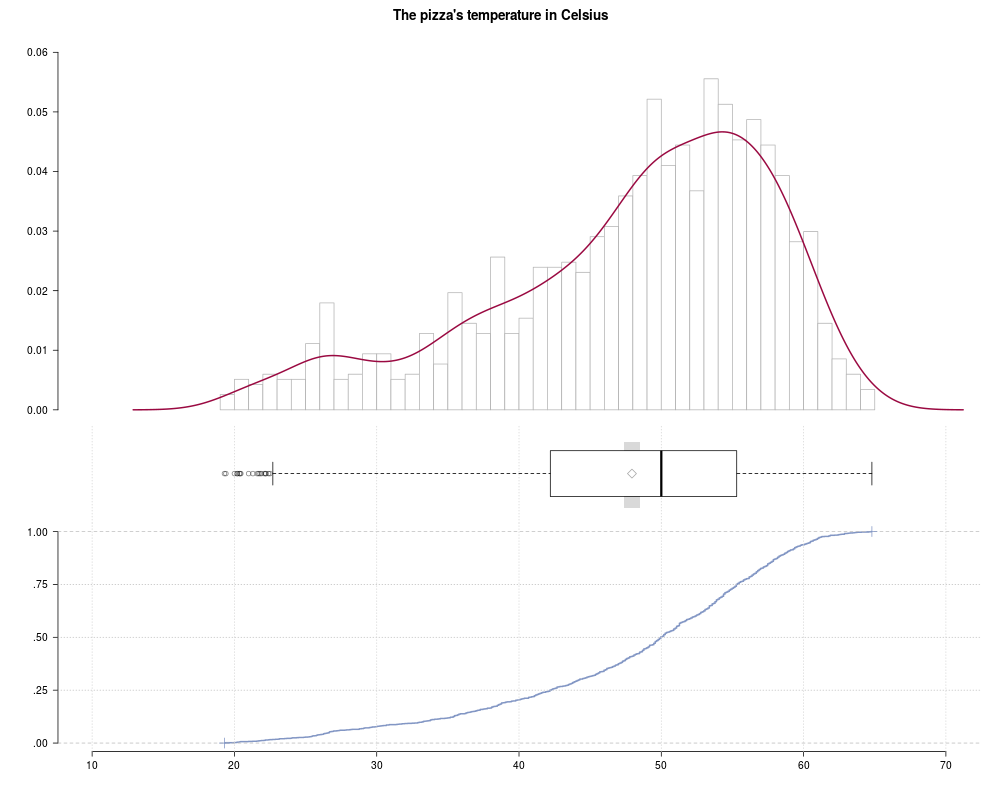
plot(z, main="The pizza's temperature in Celsius", args.hist=list(breaks=50))


# bivariate
Desc(price ~ operator, data=d.pizza)                  # numeric ~ factor
Desc(driver ~ operator, data=d.pizza)                 # factor ~ factor
Desc(driver ~ area + operator, data=d.pizza)          # factor ~ several factors
Desc(driver + area ~ operator, data=d.pizza)          # several factors ~ factor
Desc(driver ~ week, data=d.pizza)                     # factor ~ integer

Desc(driver ~ operator, data=d.pizza, rfrq=("111"))   # alle rel. frequencies
Desc(driver ~ operator, data=d.pizza, rfrq=("000"),
     verbose="high")                                  # no rel. frequencies

Desc(price ~ delivery_min, data=d.pizza)              # numeric ~ numeric
Desc(price + delivery_min ~ operator + driver + wrongpizza,
     data=d.pizza, digits=c(2,2,2,2,0,3,0,0) )

Desc(week ~ driver, data=d.pizza, digits=c(2,2,2,2,0,3,0,0))   # define digits

Desc(delivery_min + weekday ~ driver, data=d.pizza)


# without defining data-parameter
Desc(d.pizza$delivery_min ~ d.pizza$driver)


# with functions and interactions
Desc(sqrt(price) ~ operator : factor(wrongpizza), data=d.pizza)
Desc(log(price+1) ~ cut(delivery_min, breaks=seq(10,90,10)),
     data=d.pizza, digits=c(2,2,2,2,0,3,0,0))

# response versus all the rest
Desc(driver ~ ., data=d.pizza[, c("temperature","wine_delivered","area","driver")])

# all the rest versus response
Desc(. ~ driver, data=d.pizza[, c("temperature","wine_delivered","area","driver")])

# pairwise Descriptions
p <- CombPairs(c("area","count","operator","driver","temperature","wrongpizza","quality"), )
for(i in 1:nrow(p))
  print(Desc(formula(gettextf("%s ~ %s", p$X1, p$X2)), data=d.pizza))


# get more flexibility, create the table first
tab <- as.table(apply(HairEyeColor, c(1,2), sum))
tab <- tab[,c("Brown","Hazel","Green","Blue")]

# diplay only absolute values, row and columnwise percentages
Desc(tab, row.vars=c(3, 1), rfrq="011", plotit=FALSE)

# do the plot by hand, while setting the colours for the mosaics
cols1 <- SetAlpha(c("sienna4", "burlywood", "chartreuse3", "slategray1"), 0.6)
cols2 <- SetAlpha(c("moccasin", "salmon1", "wheat3", "gray32"), 0.8)
plot(tab, col1=cols1, col2=cols2)


# use global format options for presentation
options(fmt.abs=structure(list(digits=0, big.mark=""), class="fmt"))
options(fmt.per=structure(list(digits=2, fmt="%"), class="fmt"))
Desc(area ~ driver, d.pizza, plotit=FALSE)

options(fmt.abs=structure(list(digits=0, big.mark="'"), class="fmt"))
options(fmt.per=structure(list(digits=3, leading="drop"), class="fmt"))
Desc(area ~ driver, d.pizza, plotit=FALSE)

# plot arguments can be fixed in detail
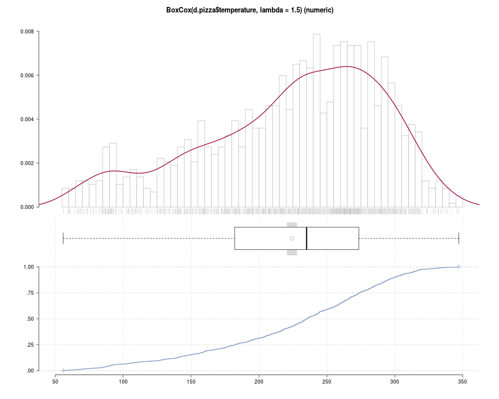
z <- Desc(BoxCox(d.pizza$temperature, lambda = 1.5))
plot(z, mar=c(0, 2.1, 4.1, 2.1), args.rug=TRUE, args.hist=list(breaks=50),
     args.dens=list(from=0))


# Output into word document (Windows-specific example) -----------------------
# by simply setting wrd=GetNewWrd()
## Not run: 

  # create a new word instance and insert title and contents
  wrd <- GetNewWrd(header=TRUE)

  # let's have a subset
  d.sub <- d.pizza[,c("driver", "date", "operator", "price", "wrongpizza")]

  # do just the univariate analysis
  Desc(d.sub, wrd=wrd)

## End(Not run)

Results


R version 3.3.1 (2016-06-21) -- "Bug in Your Hair"
Copyright (C) 2016 The R Foundation for Statistical Computing
Platform: x86_64-pc-linux-gnu (64-bit)

R is free software and comes with ABSOLUTELY NO WARRANTY.
You are welcome to redistribute it under certain conditions.
Type 'license()' or 'licence()' for distribution details.

R is a collaborative project with many contributors.
Type 'contributors()' for more information and
'citation()' on how to cite R or R packages in publications.

Type 'demo()' for some demos, 'help()' for on-line help, or
'help.start()' for an HTML browser interface to help.
Type 'q()' to quit R.

> library(DescTools)
> png(filename="/home/ddbj/snapshot/RGM3/R_CC/result/DescTools/Desc.Rd_%03d_medium.png", width=480, height=480)
> ### Name: Desc
> ### Title: Describe Data
> ### Aliases: Desc Desc.default Desc.data.frame Desc.list Desc.formula
> ###   Desc.numeric Desc.integer Desc.factor Desc.ordered Desc.character
> ###   Desc.logical Desc.Date Desc.table print.Desc plot.Desc
> ### Keywords: print univar multivariate
> 
> ### ** Examples
> 
> # implemented classes:
> Desc(d.pizza$wrongpizza)               # logical
------------------------------------------------------------------------------ 
d.pizza$wrongpizza (logical - dichotomous)

  length      n    NAs unique
   1e+03  1e+03  4e+00  2e+00

        freq   perc  lci9.50e-01  uci9.50e-01'
FALSE  1e+03  93.1%        91.5%        94.4%
TRUE   8e+01   6.9%         5.6%         8.5%

' 95%-CI Wilson

> Desc(d.pizza$driver)                   # factor
------------------------------------------------------------------------------ 
d.pizza$driver (factor)

  length      n    NAs unique levels  dupes
   1e+03  1e+03  5e+00  7e+00  7e+00      y

       level   freq   perc  cumfreq  cumperc
1  Carpenter  3e+02  22.6%    3e+02    22.6%
2     Carter  2e+02  19.4%    5e+02    42.0%
3     Taylor  2e+02  16.9%    7e+02    59.0%
4     Hunter  2e+02  13.0%    9e+02    71.9%
5     Miller  1e+02  10.4%    1e+03    82.3%
6     Farmer  1e+02   9.7%    1e+03    92.0%
7    Butcher  1e+02   8.0%    1e+03   100.0%

> Desc(d.pizza$quality)                  # ordered factor
------------------------------------------------------------------------------ 
d.pizza$quality (ordered, factor)

  length      n    NAs unique levels  dupes
   1e+03  1e+03  2e+02  3e+00  3e+00      y

    level   freq   perc  cumfreq  cumperc
1     low  2e+02  15.5%    2e+02    15.5%
2  medium  4e+02  35.3%    5e+02    50.8%
3    high  5e+02  49.2%    1e+03   100.0%

> Desc(as.character(d.pizza$driver))     # character
------------------------------------------------------------------------------ 
as.character(d.pizza$driver) (character)

  length      n    NAs unique levels  dupes
   1e+03  1e+03  5e+00  7e+00  7e+00      y

       level   freq   perc  cumfreq  cumperc
1  Carpenter  3e+02  22.6%    3e+02    22.6%
2     Carter  2e+02  19.4%    5e+02    42.0%
3     Taylor  2e+02  16.9%    7e+02    59.0%
4     Hunter  2e+02  13.0%    9e+02    71.9%
5     Miller  1e+02  10.4%    1e+03    82.3%
6     Farmer  1e+02   9.7%    1e+03    92.0%
7    Butcher  1e+02   8.0%    1e+03   100.0%

> Desc(d.pizza$week)                     # integer
------------------------------------------------------------------------------ 
d.pizza$week (numeric)

     length          n        NAs     unique         0s       mean     meanSE
      1e+03      1e+03      3e+01      6e+00          0   1.14e+01   3.87e-02

        .05        .10        .25     median        .75        .90        .95
   9.00e+00   1.00e+01   1.00e+01   1.10e+01   1.30e+01   1.30e+01   1.30e+01

      range         sd      vcoef        mad        IQR       skew       kurt
   5.00e+00   1.33e+00   1.17e-01   1.48e+00   3.00e+00  -6.74e-02  -1.01e+00
 

   level   freq   perc  cumfreq  cumperc
1      9  9e+01   7.5%    9e+01     7.5%
2     10  3e+02  21.9%    3e+02    29.4%
3     11  3e+02  22.4%    6e+02    51.8%
4     12  3e+02  22.1%    9e+02    73.9%
5     13  3e+02  23.2%    1e+03    97.1%
6     14  3e+01   2.9%    1e+03   100.0%

> Desc(d.pizza$delivery_min)             # numeric
------------------------------------------------------------------------------ 
d.pizza$delivery_min (numeric)

    length         n       NAs    unique        0s      mean    meanSE
     1e+03     1e+03         0     4e+02         0  2.57e+01  3.12e-01

       .05       .10       .25    median       .75       .90       .95
  1.04e+01  1.16e+01  1.74e+01  2.44e+01  3.25e+01  4.04e+01  4.52e+01

     range        sd     vcoef       mad       IQR      skew      kurt
  5.68e+01  1.08e+01  4.23e-01  1.13e+01  1.51e+01  6.11e-01  9.54e-02
 
lowest : 8.80e+00 (3e+00), 8.90e+00, 9.00e+00 (3e+00), 9.10e+00 (5e+00), 9.20e+00 (3e+00)
highest: 6.19e+01, 6.27e+01, 6.29e+01, 6.32e+01, 6.56e+01

> Desc(d.pizza$date)                     # Date
------------------------------------------------------------------------------ 
d.pizza$date (Date)

  length      n    NAs unique
   1e+03  1e+03  3e+01  3e+01

lowest : 2014-03-01 (42), 2014-03-02 (46), 2014-03-03 (26), 2014-03-04 (19)
highest: 2014-03-28 (46), 2014-03-29 (53), 2014-03-30 (43), 2014-03-31 (34)


Weekday:

Pearson's Chi-squared test (1-dim uniform):
  X-squared = 78.879, df = 6, p-value = 6.09e-15

       level   freq   perc  cumfreq  cumperc
1     Monday  1e+02  12.2%    1e+02    12.2%
2    Tuesday  1e+02   9.9%    3e+02    22.2%
3  Wednesday  1e+02  11.4%    4e+02    33.6%
4   Thursday  1e+02  12.5%    5e+02    46.0%
5     Friday  2e+02  14.5%    7e+02    60.6%
6   Saturday  2e+02  20.7%    1e+03    81.3%
7     Sunday  2e+02  18.7%    1e+03   100.0%

Months:

Pearson's Chi-squared test (1-dim uniform):
  X-squared = 12947, df = 11, p-value < 2.2e-16

        level   freq    perc  cumfreq  cumperc
1     January      0    0.0%        0     0.0%
2    February      0    0.0%        0     0.0%
3       March  1e+03  100.0%    1e+03   100.0%
4       April      0    0.0%    1e+03   100.0%
5         May      0    0.0%    1e+03   100.0%
6        June      0    0.0%    1e+03   100.0%
7        July      0    0.0%    1e+03   100.0%
8      August      0    0.0%    1e+03   100.0%
9   September      0    0.0%    1e+03   100.0%
10    October      0    0.0%    1e+03   100.0%
11   November      0    0.0%    1e+03   100.0%
12   December      0    0.0%    1e+03   100.0%

By days :

         level   freq  perc  cumfreq  cumperc
1   2014-03-01  4e+01  3.6%    4e+01     3.6%
2   2014-03-02  5e+01  3.9%    9e+01     7.5%
3   2014-03-03  3e+01  2.2%    1e+02     9.7%
4   2014-03-04  2e+01  1.6%    1e+02    11.3%
5   2014-03-05  3e+01  2.8%    2e+02    14.1%
6   2014-03-06  4e+01  3.3%    2e+02    17.4%
7   2014-03-07  4e+01  3.7%    2e+02    21.2%
8   2014-03-08  6e+01  4.7%    3e+02    25.8%
9   2014-03-09  4e+01  3.6%    3e+02    29.4%
10  2014-03-10  3e+01  2.2%    4e+02    31.6%
11  2014-03-11  3e+01  2.9%    4e+02    34.5%
12  2014-03-12  4e+01  3.1%    4e+02    37.6%
13  2014-03-13  4e+01  3.0%    5e+02    40.5%
14  2014-03-14  4e+01  3.2%    5e+02    43.8%
15  2014-03-15  5e+01  4.1%    6e+02    47.8%
16  2014-03-16  5e+01  4.0%    6e+02    51.8%
17  2014-03-17  3e+01  2.5%    6e+02    54.4%
18  2014-03-18  3e+01  2.7%    7e+02    57.1%
19  2014-03-19  3e+01  2.6%    7e+02    59.7%
20  2014-03-20  4e+01  3.1%    7e+02    62.8%
21  2014-03-21  4e+01  3.7%    8e+02    66.4%
22  2014-03-22  5e+01  3.9%    8e+02    70.3%
23  2014-03-23  4e+01  3.6%    9e+02    73.9%
24  2014-03-24  3e+01  2.4%    9e+02    76.3%
25  2014-03-25  3e+01  2.7%    9e+02    79.0%
26  2014-03-26  3e+01  2.9%    1e+03    81.9%
27  2014-03-27  4e+01  3.1%    1e+03    85.0%
28  2014-03-28  5e+01  3.9%    1e+03    89.0%
29  2014-03-29  5e+01  4.5%    1e+03    93.5%
30  2014-03-30  4e+01  3.7%    1e+03    97.1%
31  2014-03-31  3e+01  2.9%    1e+03   100.0%

> 
> Desc(d.pizza)
------------------------------------------------------------------------------ 
Describe data.frame

'data.frame':	1209 obs. of  16 variables:
  1 $ index         : int  1 2 3 4 5 6 7 8 9 10 ...
  2 $ date          : Date, format: "2014-03-01" "2014-03-01" "2014-03-01" "2014-03-01" ...
  3 $ week          : num  9 9 9 9 9 9 9 9 9 9 ...
  4 $ weekday       : num  6 6 6 6 6 6 6 6 6 6 ...
  5 $ area          : Factor w/ 3 levels "Brent","Camden",..: 2 3 3 1 1 2 2 1 3 1 ...
  6 $ count         : int  5 2 3 2 5 1 4 NA 3 6 ...
  7 $ rabate        : logi  TRUE FALSE FALSE FALSE TRUE FALSE ...
  8 $ price         : num  65.7 27 41 26 57.6 ...
  9 $ operator      : Factor w/ 3 levels "Allanah","Maria",..: 3 3 1 1 3 1 3 1 1 3 ...
 10 $ driver        : Factor w/ 7 levels "Butcher","Carpenter",..: 7 1 1 7 3 7 7 7 7 3 ...
 11 $ delivery_min  : num  20 19.6 17.8 37.3 21.8 48.7 49.3 25.6 26.4 24.3 ...
 12 $ temperature   : num  53 56.4 36.5 NA 50 27 33.9 54.8 48 54.4 ...
 13 $ wine_ordered  : int  0 0 0 0 0 0 1 NA 0 1 ...
 14 $ wine_delivered: int  0 0 0 0 0 0 1 NA 0 1 ...
 15 $ wrongpizza    : logi  FALSE FALSE FALSE FALSE FALSE FALSE ...
 16 $ quality       : Ord.factor w/ 3 levels "low"<"medium"<..: 2 3 NA NA 2 1 1 3 3 2 ...

------------------------------------------------------------------------------ 
1 - index (integer)

     length          n        NAs     unique         0s       mean     meanSE
      1e+03      1e+03          0        = n          0   6.05e+02   1.00e+01

        .05        .10        .25     median        .75        .90        .95
   6.14e+01   1.22e+02   3.03e+02   6.05e+02   9.07e+02   1.09e+03   1.15e+03

      range         sd      vcoef        mad        IQR       skew       kurt
   1.21e+03   3.49e+02   5.77e-01   4.48e+02   6.04e+02       0.00  -1.20e+00
 
lowest : 1e+00, 2e+00, 3e+00, 4e+00, 5e+00
highest: 1e+03, 1e+03, 1e+03, 1e+03, 1e+03

------------------------------------------------------------------------------ 
2 - date (Date)

  length      n    NAs unique
   1e+03  1e+03  3e+01  3e+01

lowest : 2014-03-01 (42), 2014-03-02 (46), 2014-03-03 (26), 2014-03-04 (19)
highest: 2014-03-28 (46), 2014-03-29 (53), 2014-03-30 (43), 2014-03-31 (34)


Weekday:

Pearson's Chi-squared test (1-dim uniform):
  X-squared = 78.879, df = 6, p-value = 6.09e-15

       level   freq   perc  cumfreq  cumperc
1     Monday  1e+02  12.2%    1e+02    12.2%
2    Tuesday  1e+02   9.9%    3e+02    22.2%
3  Wednesday  1e+02  11.4%    4e+02    33.6%
4   Thursday  1e+02  12.5%    5e+02    46.0%
5     Friday  2e+02  14.5%    7e+02    60.6%
6   Saturday  2e+02  20.7%    1e+03    81.3%
7     Sunday  2e+02  18.7%    1e+03   100.0%

Months:

Pearson's Chi-squared test (1-dim uniform):
  X-squared = 12947, df = 11, p-value < 2.2e-16

        level   freq    perc  cumfreq  cumperc
1     January      0    0.0%        0     0.0%
2    February      0    0.0%        0     0.0%
3       March  1e+03  100.0%    1e+03   100.0%
4       April      0    0.0%    1e+03   100.0%
5         May      0    0.0%    1e+03   100.0%
6        June      0    0.0%    1e+03   100.0%
7        July      0    0.0%    1e+03   100.0%
8      August      0    0.0%    1e+03   100.0%
9   September      0    0.0%    1e+03   100.0%
10    October      0    0.0%    1e+03   100.0%
11   November      0    0.0%    1e+03   100.0%
12   December      0    0.0%    1e+03   100.0%

By days :

         level   freq  perc  cumfreq  cumperc
1   2014-03-01  4e+01  3.6%    4e+01     3.6%
2   2014-03-02  5e+01  3.9%    9e+01     7.5%
3   2014-03-03  3e+01  2.2%    1e+02     9.7%
4   2014-03-04  2e+01  1.6%    1e+02    11.3%
5   2014-03-05  3e+01  2.8%    2e+02    14.1%
6   2014-03-06  4e+01  3.3%    2e+02    17.4%
7   2014-03-07  4e+01  3.7%    2e+02    21.2%
8   2014-03-08  6e+01  4.7%    3e+02    25.8%
9   2014-03-09  4e+01  3.6%    3e+02    29.4%
10  2014-03-10  3e+01  2.2%    4e+02    31.6%
11  2014-03-11  3e+01  2.9%    4e+02    34.5%
12  2014-03-12  4e+01  3.1%    4e+02    37.6%
13  2014-03-13  4e+01  3.0%    5e+02    40.5%
14  2014-03-14  4e+01  3.2%    5e+02    43.8%
15  2014-03-15  5e+01  4.1%    6e+02    47.8%
16  2014-03-16  5e+01  4.0%    6e+02    51.8%
17  2014-03-17  3e+01  2.5%    6e+02    54.4%
18  2014-03-18  3e+01  2.7%    7e+02    57.1%
19  2014-03-19  3e+01  2.6%    7e+02    59.7%
20  2014-03-20  4e+01  3.1%    7e+02    62.8%
21  2014-03-21  4e+01  3.7%    8e+02    66.4%
22  2014-03-22  5e+01  3.9%    8e+02    70.3%
23  2014-03-23  4e+01  3.6%    9e+02    73.9%
24  2014-03-24  3e+01  2.4%    9e+02    76.3%
25  2014-03-25  3e+01  2.7%    9e+02    79.0%
26  2014-03-26  3e+01  2.9%    1e+03    81.9%
27  2014-03-27  4e+01  3.1%    1e+03    85.0%
28  2014-03-28  5e+01  3.9%    1e+03    89.0%
29  2014-03-29  5e+01  4.5%    1e+03    93.5%
30  2014-03-30  4e+01  3.7%    1e+03    97.1%
31  2014-03-31  3e+01  2.9%    1e+03   100.0%

------------------------------------------------------------------------------ 
3 - week (numeric)

     length          n        NAs     unique         0s       mean     meanSE
      1e+03      1e+03      3e+01      6e+00          0   1.14e+01   3.87e-02

        .05        .10        .25     median        .75        .90        .95
   9.00e+00   1.00e+01   1.00e+01   1.10e+01   1.30e+01   1.30e+01   1.30e+01

      range         sd      vcoef        mad        IQR       skew       kurt
   5.00e+00   1.33e+00   1.17e-01   1.48e+00   3.00e+00  -6.74e-02  -1.01e+00
 

   level   freq   perc  cumfreq  cumperc
1      9  9e+01   7.5%    9e+01     7.5%
2     10  3e+02  21.9%    3e+02    29.4%
3     11  3e+02  22.4%    6e+02    51.8%
4     12  3e+02  22.1%    9e+02    73.9%
5     13  3e+02  23.2%    1e+03    97.1%
6     14  3e+01   2.9%    1e+03   100.0%

------------------------------------------------------------------------------ 
4 - weekday (numeric)

     length          n        NAs     unique         0s       mean     meanSE
      1e+03      1e+03      3e+01      7e+00          0   4.44e+00   5.89e-02

        .05        .10        .25     median        .75        .90        .95
   1.00e+00   1.00e+00   3.00e+00   5.00e+00   6.00e+00   7.00e+00   7.00e+00

      range         sd      vcoef        mad        IQR       skew       kurt
   6.00e+00   2.02e+00   4.55e-01   2.97e+00   3.00e+00  -3.45e-01  -1.17e+00
 

   level   freq   perc  cumfreq  cumperc
1      1  1e+02  12.2%    1e+02    12.2%
2      2  1e+02   9.9%    3e+02    22.2%
3      3  1e+02  11.4%    4e+02    33.6%
4      4  1e+02  12.5%    5e+02    46.0%
5      5  2e+02  14.5%    7e+02    60.6%
6      6  2e+02  20.7%    1e+03    81.3%
7      7  2e+02  18.7%    1e+03   100.0%

------------------------------------------------------------------------------ 
5 - area (factor)

  length      n    NAs unique levels  dupes
   1e+03  1e+03  1e+01  3e+00  3e+00      y

         level   freq   perc  cumfreq  cumperc
1        Brent  5e+02  39.5%    5e+02    39.5%
2  Westminster  4e+02  31.8%    9e+02    71.3%
3       Camden  3e+02  28.7%    1e+03   100.0%

------------------------------------------------------------------------------ 
6 - count (integer)

     length          n        NAs     unique         0s       mean     meanSE
      1e+03      1e+03      1e+01      8e+00          0   3.44e+00   4.50e-02

        .05        .10        .25     median        .75        .90        .95
   1.00e+00   2.00e+00   2.00e+00   3.00e+00   4.00e+00   6.00e+00   6.00e+00

      range         sd      vcoef        mad        IQR       skew       kurt
   7.00e+00   1.56e+00   4.52e-01   1.48e+00   2.00e+00   4.54e-01  -3.63e-01
 

   level   freq   perc  cumfreq  cumperc
1      1  1e+02   9.0%    1e+02     9.0%
2      2  3e+02  21.6%    4e+02    30.7%
3      3  3e+02  25.1%    7e+02    55.7%
4      4  2e+02  20.1%    9e+02    75.8%
5      5  2e+02  12.7%    1e+03    88.5%
6      6  1e+02   8.1%    1e+03    96.6%
7      7  3e+01   2.8%    1e+03    99.4%
8      8  7e+00   0.6%    1e+03   100.0%

------------------------------------------------------------------------------ 
7 - rabate (logical - dichotomous)

  length      n    NAs unique
   1e+03  1e+03  1e+01  2e+00

        freq   perc  lci9.50e-01  uci9.50e-01'
FALSE  6e+02  50.2%        47.4%        53.0%
TRUE   6e+02  49.8%        47.0%        52.6%

' 95%-CI Wilson

------------------------------------------------------------------------------ 
8 - price (numeric)

      length           n         NAs      unique          0s        mean      meanSE
       1e+03       1e+03       1e+01       4e+02           0  4.8729e+01  6.2522e-01

         .05         .10         .25      median         .75         .90         .95
  1.3990e+01  2.3980e+01  3.0980e+01  4.6764e+01  6.3180e+01  7.8833e+01  8.7120e+01

       range          sd       vcoef         mad         IQR        skew        kurt
  1.2554e+02  2.1631e+01  4.4391e-01  2.3401e+01  3.2200e+01  4.9708e-01  1.0761e-01
 
lowest : 8.7920e+00 (3e+00), 9.5920e+00, 1.0392e+01 (2e+00), 1.0990e+01 (1e+01), 1.1192e+01 (2e+00)
highest: 1.1653e+02, 1.2339e+02, 1.2443e+02, 1.2955e+02, 1.3433e+02

------------------------------------------------------------------------------ 
9 - operator (factor)

  length      n    NAs unique levels  dupes
   1e+03  1e+03  8e+00  3e+00  3e+00      y

     level   freq   perc  cumfreq  cumperc
1   Rhonda  4e+02  37.1%    4e+02    37.1%
2    Maria  4e+02  32.3%    8e+02    69.4%
3  Allanah  4e+02  30.6%    1e+03   100.0%

------------------------------------------------------------------------------ 
10 - driver (factor)

  length      n    NAs unique levels  dupes
   1e+03  1e+03  5e+00  7e+00  7e+00      y

       level   freq   perc  cumfreq  cumperc
1  Carpenter  3e+02  22.6%    3e+02    22.6%
2     Carter  2e+02  19.4%    5e+02    42.0%
3     Taylor  2e+02  16.9%    7e+02    59.0%
4     Hunter  2e+02  13.0%    9e+02    71.9%
5     Miller  1e+02  10.4%    1e+03    82.3%
6     Farmer  1e+02   9.7%    1e+03    92.0%
7    Butcher  1e+02   8.0%    1e+03   100.0%

------------------------------------------------------------------------------ 
11 - delivery_min (numeric)

    length         n       NAs    unique        0s      mean    meanSE
     1e+03     1e+03         0     4e+02         0  2.57e+01  3.12e-01

       .05       .10       .25    median       .75       .90       .95
  1.04e+01  1.16e+01  1.74e+01  2.44e+01  3.25e+01  4.04e+01  4.52e+01

     range        sd     vcoef       mad       IQR      skew      kurt
  5.68e+01  1.08e+01  4.23e-01  1.13e+01  1.51e+01  6.11e-01  9.54e-02
 
lowest : 8.80e+00 (3e+00), 8.90e+00, 9.00e+00 (3e+00), 9.10e+00 (5e+00), 9.20e+00 (3e+00)
highest: 6.19e+01, 6.27e+01, 6.29e+01, 6.32e+01, 6.56e+01

------------------------------------------------------------------------------ 
12 - temperature (numeric)

      length           n         NAs      unique          0s        mean      meanSE
       1e+03       1e+03       4e+01       4e+02           0   4.794e+01   2.905e-01

         .05         .10         .25      median         .75         .90         .95
   2.670e+01   3.329e+01   4.223e+01   5.000e+01   5.530e+01   5.880e+01   6.050e+01

       range          sd       vcoef         mad         IQR        skew        kurt
   4.550e+01   9.938e+00   2.073e-01   9.192e+00   1.307e+01  -8.419e-01   5.058e-02
 
lowest : 1.930e+01, 1.940e+01, 2.000e+01, 2.020e+01 (2e+00), 2.035e+01
highest: 6.380e+01, 6.410e+01, 6.460e+01, 6.470e+01, 6.480e+01

------------------------------------------------------------------------------ 
13 - wine_ordered (integer - dichotomous)

  length      n    NAs unique
   1e+03  1e+03  1e+01  2e+00

    freq   perc  lci9.50e-01  uci9.50e-01'
0  1e+03  84.4%        82.2%        86.3%
1  2e+02  15.6%        13.7%        17.8%

' 95%-CI Wilson

------------------------------------------------------------------------------ 
14 - wine_delivered (integer - dichotomous)

  length      n    NAs unique
   1e+03  1e+03  1e+01  2e+00

    freq   perc  lci9.50e-01  uci9.50e-01'
0  1e+03  86.4%        84.3%        88.2%
1  2e+02  13.6%        11.8%        15.7%

' 95%-CI Wilson

------------------------------------------------------------------------------ 
15 - wrongpizza (logical - dichotomous)

  length      n    NAs unique
   1e+03  1e+03  4e+00  2e+00

        freq   perc  lci9.50e-01  uci9.50e-01'
FALSE  1e+03  93.1%        91.5%        94.4%
TRUE   8e+01   6.9%         5.6%         8.5%

' 95%-CI Wilson

------------------------------------------------------------------------------ 
16 - quality (ordered, factor)

  length      n    NAs unique levels  dupes
   1e+03  1e+03  2e+02  3e+00  3e+00      y

    level   freq   perc  cumfreq  cumperc
1     low  2e+02  15.5%    2e+02    15.5%
2  medium  4e+02  35.3%    5e+02    50.8%
3    high  5e+02  49.2%    1e+03   100.0%

> 
> Desc(d.pizza$wrongpizza, main="The wrong pizza delivered", digits=5)
------------------------------------------------------------------------------ 
The wrong pizza delivered

  length      n    NAs unique
   1e+03  1e+03  4e+00  2e+00

        freq       perc  lci9.50e-01  uci9.50e-01'
FALSE  1e+03  93.11203%    91.54086%    94.40921%
TRUE   8e+01   6.88797%     5.59079%     8.45914%

' 95%-CI Wilson

> 
> Desc(table(d.pizza$area))                                    # 1-dim table
------------------------------------------------------------------------------ 
table(d.pizza$area) (table)

Summary: 
n: 1e+03, rows: 3

Pearson's Chi-squared test (1-dim uniform):
  X-squared = 22.45, df = 2, p-value = 1.333e-05

         level   freq   perc  cumfreq  cumperc
1        Brent  5e+02  39.5%    5e+02    39.5%
2       Camden  3e+02  28.7%    8e+02    68.2%
3  Westminster  4e+02  31.8%    1e+03   100.0%

> Desc(table(d.pizza$area, d.pizza$operator))                  # 2-dim table
------------------------------------------------------------------------------ 
table(d.pizza$area, d.pizza$operator) (table)

Summary: 
n: 1e+03, rows: 3e+00, columns: 3e+00

Pearson's Chi-squared test:
  X-squared = 17.905, df = 4, p-value = 0.001288
Likelihood Ratio:
  X-squared = 18.099, df = 4, p-value = 0.001181
Mantel-Haenszel Chi-squared:
  X-squared = 8.6654, df = 1, p-value = 0.003243

Phi-Coefficient        0.123
Contingency Coeff.     0.122
Cramer's V             0.087

                   
                   Allanah  Maria Rhonda    Sum
                                               
Brent       freq     2e+02  2e+02  2e+02  5e+02
            perc     12.8%  12.8%  14.0%  39.7%
            p.row    32.3%  32.3%  35.3%      .
            p.col    41.9%  39.9%  37.7%      .

Camden      freq     1e+02  1e+02  1e+02  3e+02
            perc     10.3%   9.1%   9.2%  28.5%
            p.row    36.2%  31.8%  32.1%      .
            p.col    33.7%  28.2%  24.6%      .

Westminster freq     9e+01  1e+02  2e+02  4e+02
            perc      7.5%  10.2%  14.0%  31.7%
            p.row    23.5%  32.3%  44.2%      .
            p.col    24.4%  31.9%  37.7%      .

Sum         freq     4e+02  4e+02  4e+02  1e+03
            perc     30.6%  32.2%  37.2% 100.0%
            p.row        .      .      .      .
            p.col        .      .      .      .

> Desc(table(d.pizza$area, d.pizza$operator, d.pizza$driver))  # n-dim table
------------------------------------------------------------------------------ 
table(d.pizza$area, d.pizza$operator, d.pizza$driver) (table)

Summary: 
n: 1e+03, 3-dim table: 3 x 3 x 7

Chi-squared test for independence of all factors:
  X-squared = 1.253e+03, df = 52, p-value = < 2.2e-16

                     Butcher Carpenter Carter Farmer Hunter Miller Taylor Sum
                                                                             
Brent       Allanah       24         6     36      5     56      2     23 152
            Maria          5        10     89      5     35      1      8 153
            Rhonda        43        13     52      8     37      3     11 167
Camden      Allanah        0         4     16     21      0     11     69 121
            Maria          0         5     22     31      1     18     31 108
            Rhonda         1        10      9     35      3     10     40 108
Westminster Allanah        6        47      2      2     12     12      7  88
            Maria          3        71      3      2      7     30      6 122
            Rhonda        13       101      0      7      5     34      7 167
Sum         Allanah       30        57     54     28     68     25     99 361
            Maria          8        86    114     38     43     49     45 383
            Rhonda        57       124     61     50     45     47     58 442

> 
> # expressions
> Desc(log(d.pizza$temperature))
------------------------------------------------------------------------------ 
log(d.pizza$temperature) (numeric)

         length              n            NAs         unique             0s           mean         meanSE
          1e+03          1e+03          4e+01          4e+02              0   3.843745e+00   7.061375e-03

            .05            .10            .25         median            .75            .90            .95
   3.284664e+00   3.505257e+00   3.743012e+00   3.912023e+00   4.012773e+00   4.074142e+00   4.102643e+00

          range             sd          vcoef            mad            IQR           skew           kurt
   1.211201e+00   2.415362e-01   6.283876e-02   1.811999e-01   2.697610e-01  -1.377446e+00   1.528453e+00
 
lowest : 2.960105e+00, 2.965273e+00, 2.995732e+00, 3.005683e+00 (2e+00), 3.013081e+00
highest: 4.155753e+00, 4.160444e+00, 4.168214e+00, 4.169761e+00, 4.171306e+00

> Desc(d.pizza$temperature > 45)
------------------------------------------------------------------------------ 
d.pizza$temperature > 45 (logical - dichotomous)

  length      n    NAs unique
   1e+03  1e+03  4e+01  2e+00

        freq   perc  lci9.50e-01  uci9.50e-01'
TRUE   8e+02  68.5%        65.7%        71.1%
FALSE  4e+02  31.5%        28.9%        34.3%

' 95%-CI Wilson

> 
> # supported labels
> Label(d.pizza$temperature) <- "This is the temperature in degrees Celsius
+ measured at the time when the pizza is delivered to the client."
> Desc(d.pizza$temperature)
------------------------------------------------------------------------------ 
d.pizza$temperature (numeric) :
  This is the temperature in degrees Celsius measured at the time when
  the pizza is delivered to the client.


      length           n         NAs      unique          0s        mean      meanSE
       1e+03       1e+03       4e+01       4e+02           0   4.794e+01   2.905e-01

         .05         .10         .25      median         .75         .90         .95
   2.670e+01   3.329e+01   4.223e+01   5.000e+01   5.530e+01   5.880e+01   6.050e+01

       range          sd       vcoef         mad         IQR        skew        kurt
   4.550e+01   9.938e+00   2.073e-01   9.192e+00   1.307e+01  -8.419e-01   5.058e-02
 
lowest : 1.930e+01, 1.940e+01, 2.000e+01, 2.020e+01 (2e+00), 2.035e+01
highest: 6.380e+01, 6.410e+01, 6.460e+01, 6.470e+01, 6.480e+01

> # try as well:      Desc(d.pizza$temperature, wrd=GetNewWrd())
> 
> z <- Desc(d.pizza$temperature)
> print(z, digits=1, plotit=FALSE)
------------------------------------------------------------------------------ 
d.pizza$temperature (numeric) :
  This is the temperature in degrees Celsius measured at the time when
  the pizza is delivered to the client.


    length         n       NAs    unique        0s      mean    meanSE
     1e+03     1e+03     4e+01     4e+02         0   4.8e+01   2.9e-01

       .05       .10       .25    median       .75       .90       .95
   2.7e+01   3.3e+01   4.2e+01   5.0e+01   5.5e+01   5.9e+01   6.0e+01

     range        sd     vcoef       mad       IQR      skew      kurt
   4.6e+01   9.9e+00   2.1e-01   9.2e+00   1.3e+01  -8.4e-01   5.1e-02
 
lowest : 1.9e+01, 1.9e+01, 2.0e+01, 2.0e+01 (2e+00), 2.0e+01
highest: 6.4e+01, 6.4e+01, 6.5e+01, 6.5e+01, 6.5e+01

> # plot (additional arguments are passed on to the underlying plot function)
> plot(z, main="The pizza's temperature in Celsius", args.hist=list(breaks=50))
> 
> 
> # bivariate
> Desc(price ~ operator, data=d.pizza)                  # numeric ~ factor
------------------------------------------------------------------------------ 
price ~ operator

Summary: 
n pairs: 1e+03, valid: 1e+03 (98.3%), missings: 2e+01 (1.7%), groups: 3

                                       
          Allanah      Maria     Rhonda
mean    4.631e+01  4.912e+01  5.037e+01
median  4.497e+01  4.676e+01  4.797e+01
sd      2.015e+01  2.198e+01  2.241e+01
IQR     2.887e+01  3.183e+01  3.343e+01
n           4e+02      4e+02      4e+02
np        30.530%    32.296%    37.174%
NAs         4e+00      4e+00      4e+00
0s              0          0          0

Kruskal-Wallis rank sum test:
  Kruskal-Wallis chi-squared = 6.2048, df = 2, p-value = 0.04494
Warning:
  Grouping variable contains 8 NAs (0.662%).

> Desc(driver ~ operator, data=d.pizza)                 # factor ~ factor
------------------------------------------------------------------------------ 
driver ~ operator


Summary: 
n: 1e+03, rows: 7e+00, columns: 3e+00

Pearson's Chi-squared test:
  X-squared = 133.06, df = 12, p-value < 2.2e-16
Likelihood Ratio:
  X-squared = 133.53, df = 12, p-value < 2.2e-16
Mantel-Haenszel Chi-squared:
  X-squared = 33.539, df = 1, p-value = 6.984e-09

Phi-Coefficient        0.334
Contingency Coeff.     0.316
Cramer's V             0.236

                 operator
                 Allanah  Maria Rhonda    Sum
driver                                       

Butcher   freq     3e+01  8e+00  6e+01  1e+02
          perc      2.5%   0.7%   4.8%   8.0%
          p.row    31.2%   8.3%  60.4%      .
          p.col     8.3%   2.1%  13.0%      .

Carpenter freq     6e+01  9e+01  1e+02  3e+02
          perc      4.8%   7.3%  10.5%  22.6%
          p.row    21.5%  32.2%  46.3%      .
          p.col    16.0%  22.4%  28.1%      .

Carter    freq     6e+01  1e+02  6e+01  2e+02
          perc      4.6%   9.8%   5.2%  19.6%
          p.row    23.5%  50.0%  26.5%      .
          p.col    15.2%  3