R Graphical Manual

Browse All

Last data update: 2014.03.03

R: Plot a Correlation Matrix

PlotCorr

R Documentation

Plot a Correlation Matrix

Description

This function produces a graphical display of a correlation matrix. The cells of the matrix can be shaded or colored to show the correlation value.

Usage

PlotCorr(x, cols = colorRampPalette(c(getOption("col1", hred), "white",
                                      getOption("col2", hblue)), space = "rgb")(20),
         breaks = seq(-1, 1, length = length(cols) + 1),
         border = "grey", lwd = 1,
         args.colorlegend = NULL, xaxt = par("xaxt"), yaxt = par("yaxt"),
         cex.axis = 0.8, las = 2, mar = c(3, 8, 8, 8), ...)

Arguments

`x`	x is a correlation matrix to be visualized.
`cols`	the colors for shading the matrix. Uses the package's option `"col1"` and `"col2"` as default.
`breaks`	a set of breakpoints for the colours: must give one more breakpoint than colour. These are passed to `image()` function. If breaks is specified then the algorithm used follows `cut`, so intervals are closed on the right and open on the left except for the lowest interval.
`border`	color for borders. The default is `grey`. Set this argument to `NA` if borders should be omitted.
`lwd`	line width for borders. Default is 1.
`args.colorlegend`	list of arguments for the `ColorLegend`. Use NA if no color legend should be painted.
`xaxt`	parameter to define, whether to draw an x-axis, defaults to `"n"`.
`yaxt`	parameter to define, whether to draw an y-axis, defaults to `"n"`.
`cex.axis`	character extension for the axis labels.
`las`	the style of axis labels.
`mar`	sets the margins, defaults to mar = c(3, 8, 8, 8) as we need a bit more room on the right.
`...`	the dots are passed to the function `image`, which produces the plot.

Value

no values returned.

Author(s)

Andri Signorell <andri@signorell.net>

Examples

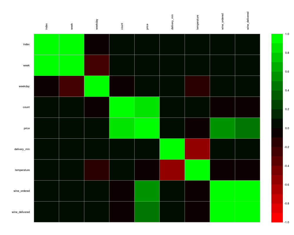
m <- cor(d.pizza[,sapply(d.pizza, IsNumeric, na.rm=TRUE)], use="pairwise.complete.obs")

PlotCorr(m, cols=colorRampPalette(c("red", "black", "green"), space = "rgb")(20))
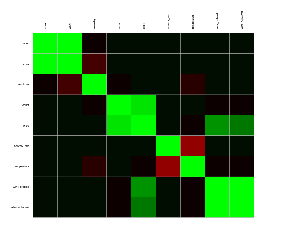
PlotCorr(m, cols=colorRampPalette(c("red", "black", "green"), space = "rgb")(20),
         args.colorlegend=NA)

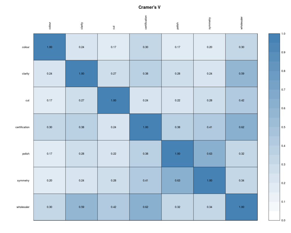
m <- PairApply(d.diamonds[, sapply(d.diamonds, is.factor)], CramerV, symmetric=TRUE)
PlotCorr(m, cols = colorRampPalette(c("white", "steelblue"), space = "rgb")(20),
         breaks=seq(0, 1, length=21), border="black",
         args.colorlegend = list(labels=sprintf("%.1f", seq(0, 1, length = 11)), frame=TRUE)
)
title(main="Cramer's V", line=2)
text(x=rep(1:ncol(m),ncol(m)), y=rep(1:ncol(m),each=ncol(m)),
     label=sprintf("%0.2f", m[,ncol(m):1]), cex=0.8, xpd=TRUE)

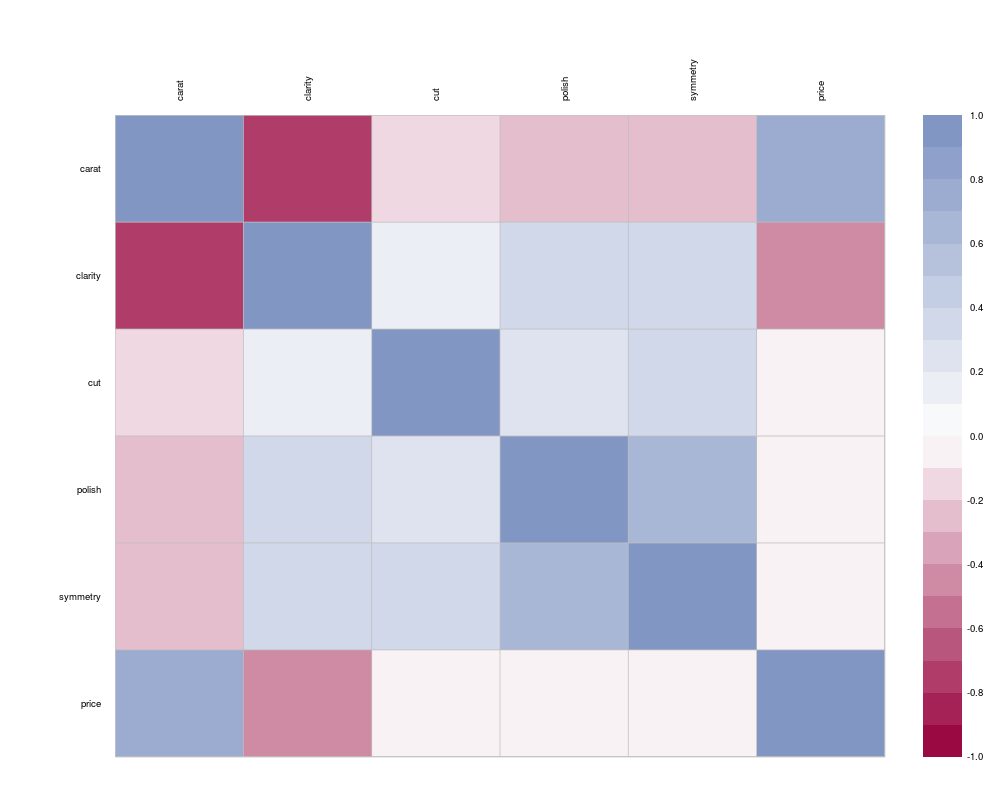
# Spearman correlation on ordinal factors
csp <- cor(data.frame(lapply(d.diamonds[,c("carat", "clarity", "cut", "polish",
                      "symmetry", "price")], as.numeric)), method="spearman")
PlotCorr(csp)

# some more colors
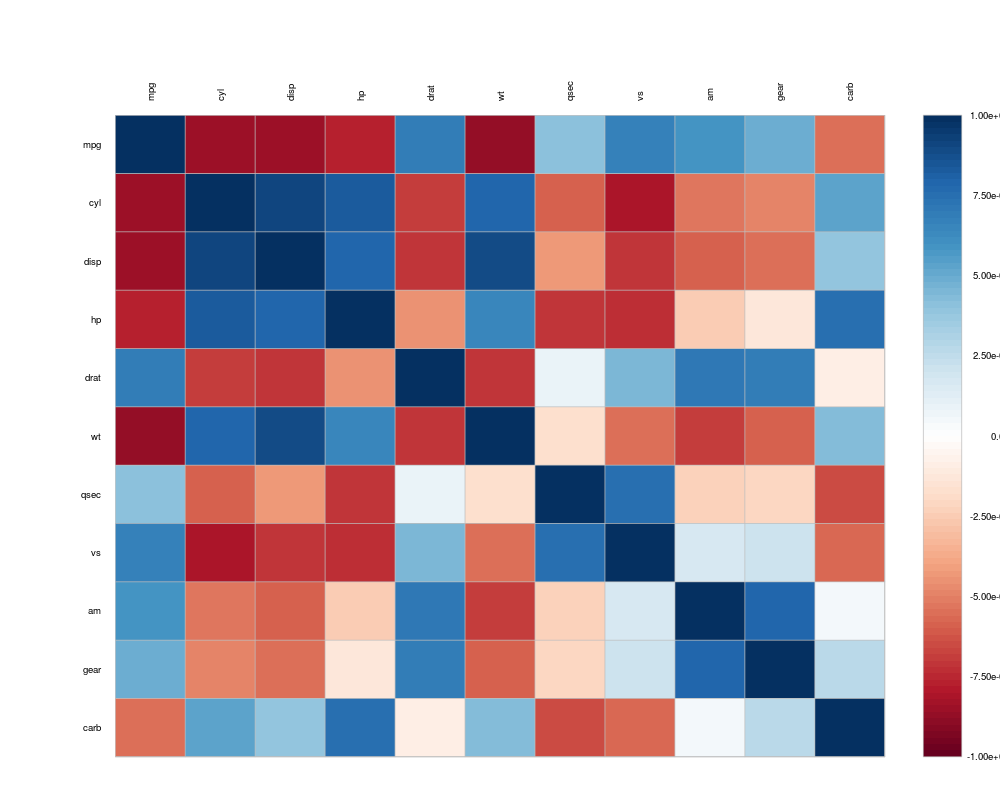
PlotCorr(cor(mtcars), col=PalDescTools("RedWhiteBlue1", 100), border="grey",
         args.colorlegend=list(labels=Format(seq(-1,1,.25), digits=2), frame="grey"))

Results


R version 3.3.1 (2016-06-21) -- "Bug in Your Hair"
Copyright (C) 2016 The R Foundation for Statistical Computing
Platform: x86_64-pc-linux-gnu (64-bit)

R is free software and comes with ABSOLUTELY NO WARRANTY.
You are welcome to redistribute it under certain conditions.
Type 'license()' or 'licence()' for distribution details.

R is a collaborative project with many contributors.
Type 'contributors()' for more information and
'citation()' on how to cite R or R packages in publications.

Type 'demo()' for some demos, 'help()' for on-line help, or
'help.start()' for an HTML browser interface to help.
Type 'q()' to quit R.

> library(DescTools)
> png(filename="/home/ddbj/snapshot/RGM3/R_CC/result/DescTools/PlotCorr.Rd_%03d_medium.png", width=480, height=480)
> ### Name: PlotCorr
> ### Title: Plot a Correlation Matrix
> ### Aliases: PlotCorr
> ### Keywords: hplot multivariate
> 
> ### ** Examples
> 
> m <- cor(d.pizza[,sapply(d.pizza, IsNumeric, na.rm=TRUE)], use="pairwise.complete.obs")
> 
> PlotCorr(m, cols=colorRampPalette(c("red", "black", "green"), space = "rgb")(20))
> PlotCorr(m, cols=colorRampPalette(c("red", "black", "green"), space = "rgb")(20),
+          args.colorlegend=NA)
> 
> m <- PairApply(d.diamonds[, sapply(d.diamonds, is.factor)], CramerV, symmetric=TRUE)
> PlotCorr(m, cols = colorRampPalette(c("white", "steelblue"), space = "rgb")(20),
+          breaks=seq(0, 1, length=21), border="black",
+          args.colorlegend = list(labels=sprintf("%.1f", seq(0, 1, length = 11)), frame=TRUE)
+ )
> title(main="Cramer's V", line=2)
> text(x=rep(1:ncol(m),ncol(m)), y=rep(1:ncol(m),each=ncol(m)),
+      label=sprintf("%0.2f", m[,ncol(m):1]), cex=0.8, xpd=TRUE)
> 
> # Spearman correlation on ordinal factors
> csp <- cor(data.frame(lapply(d.diamonds[,c("carat", "clarity", "cut", "polish",
+                       "symmetry", "price")], as.numeric)), method="spearman")
> PlotCorr(csp)
> 
> # some more colors
> PlotCorr(cor(mtcars), col=PalDescTools("RedWhiteBlue1", 100), border="grey",
+          args.colorlegend=list(labels=Format(seq(-1,1,.25), digits=2), frame="grey"))
> 
> 
> 
> 
> 
> dev.off()
null device 
          1 
>