Supported by Dr. Osamu Ogasawara and  . . |
|
Last data update: 2014.03.03 |
Draw a Back To Back Pyramid PlotDescriptionPyramid plots are a common way to display the distribution of age groups. Usage
PlotPyramid(lx, rx = NA, ylab = "", ylab.x = 0,
            col = c("red", "blue"), border = par("fg"),
            main = "", lxlab = "", rxlab = "",
            xlim = NULL, gapwidth = NULL,
            xaxt = TRUE, args.grid = NULL, cex.axis = par("cex.axis"),
            cex.lab = par("cex.axis"), cex.names = par("cex.axis"), adj = 0.5, ...)
Arguments
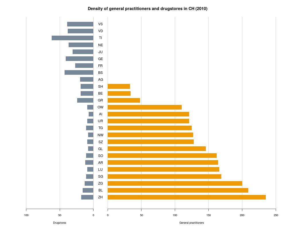
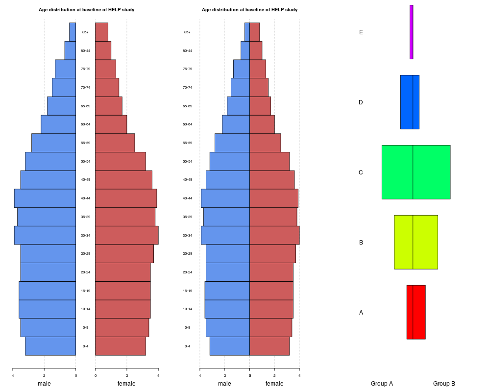
DetailsPyramid plots are a common way to display the distribution of age groups in a human population. The percentages of people within a given age category are arranged in a barplot, typically back to back. Such displays can be used to distinguish males vs. females, differences between two different countries or the distribution of age at different timepoints. The plot type can also be used to display other types of opposed bar charts with suitable modification of the arguments. ValueA numeric vector giving the coordinates of all the bar midpoints drawn, useful for adding to the graph. Author(s)Andri Signorell <andri@signorell.net> See Also
Examples
d.sda <- data.frame(
  kt_x =  c("ZH","BL","ZG","SG","LU","AR","SO","GL","SZ",
            "NW","TG","UR","AI","OW","GR","BE","SH","AG",
            "BS","FR","GE","JU","NE","TI","VD","VS"),
  apo_n = c(18,16,13,11,9,12,11,8,9,8,11,9,7,9,24,19,
            19,20,43,27,41,31,37,62,38,39),
  sda_n = c(235,209,200,169,166,164,162,146,128,127,
            125,121,121,110,48,34,33,0,0,0,0,0,0,0,0,0)
)

PlotPyramid(lx=d.sda[,c("apo_n","sda_n")], ylab=d.sda$kt_x,
            col=c("lightslategray", "orange2"), border = NA, ylab.x=0,
            xlim=c(-110,250),
            gapwidth = NULL, cex.lab = 0.8, cex.axis=0.8, xaxt = TRUE,
            lxlab="Drugstores", rxlab="General practitioners",
            main="Density of general practitioners and drugstores in CH (2010)",
            space=0.5, args.grid=list(lty=1))


par(mfrow=c(1,3))

m.pop<-c(3.2,3.5,3.6,3.6,3.5,3.5,3.9,3.7,3.9,3.5,
         3.2,2.8,2.2,1.8,1.5,1.3,0.7,0.4)
f.pop<-c(3.2,3.4,3.5,3.5,3.5,3.7,4,3.8,3.9,3.6,3.2,
         2.5,2,1.7,1.5,1.3,1,0.8)
age <- c("0-4","5-9","10-14","15-19","20-24","25-29",
         "30-34","35-39","40-44","45-49","50-54",
         "55-59","60-64","65-69","70-74","75-79","80-44","85+")

PlotPyramid(m.pop, f.pop,
            ylab = age, space = 0, col = c("cornflowerblue", "indianred"),
            main="Age distribution at baseline of HELP study",
            lxlab="male", rxlab="female" )

PlotPyramid(m.pop, f.pop,
            ylab = age, space = 0, col = c("cornflowerblue", "indianred"),
            xlim=c(-5,5),
            main="Age distribution at baseline of HELP study",
            lxlab="male", rxlab="female", gapwidth=0, ylab.x=-5 )


PlotPyramid(c(1,3,5,2,0.5), c(2,4,6,1,0),
            ylab = LETTERS[1:5], space = 0.3, col = rep(rainbow(5), each=2),
            xlim=c(-10,10), args.grid=NA, cex.names=1.5, adj=1,
            lxlab="Group A", rxlab="Group B", gapwidth=0, ylab.x=-8, xaxt="n")
Results
R version 3.3.1 (2016-06-21) -- "Bug in Your Hair"
Copyright (C) 2016 The R Foundation for Statistical Computing
Platform: x86_64-pc-linux-gnu (64-bit)

R is free software and comes with ABSOLUTELY NO WARRANTY.
You are welcome to redistribute it under certain conditions.
Type 'license()' or 'licence()' for distribution details.

R is a collaborative project with many contributors.
Type 'contributors()' for more information and
'citation()' on how to cite R or R packages in publications.

Type 'demo()' for some demos, 'help()' for on-line help, or
'help.start()' for an HTML browser interface to help.
Type 'q()' to quit R.

> library(DescTools)
> png(filename="/home/ddbj/snapshot/RGM3/R_CC/result/DescTools/PlotPyramid.Rd_%03d_medium.png", width=480, height=480)
> ### Name: PlotPyramid
> ### Title: Draw a Back To Back Pyramid Plot
> ### Aliases: PlotPyramid
> ### Keywords: hplot
>
> ### ** Examples
>
> d.sda <- data.frame(
+   kt_x =  c("ZH","BL","ZG","SG","LU","AR","SO","GL","SZ",
+             "NW","TG","UR","AI","OW","GR","BE","SH","AG",
+             "BS","FR","GE","JU","NE","TI","VD","VS"),
+   apo_n = c(18,16,13,11,9,12,11,8,9,8,11,9,7,9,24,19,
+             19,20,43,27,41,31,37,62,38,39),
+   sda_n = c(235,209,200,169,166,164,162,146,128,127,
+             125,121,121,110,48,34,33,0,0,0,0,0,0,0,0,0)
+ )
>
> PlotPyramid(lx=d.sda[,c("apo_n","sda_n")], ylab=d.sda$kt_x,
+             col=c("lightslategray", "orange2"), border = NA, ylab.x=0,
+             xlim=c(-110,250),
+             gapwidth = NULL, cex.lab = 0.8, cex.axis=0.8, xaxt = TRUE,
+             lxlab="Drugstores", rxlab="General practitioners",
+             main="Density of general practitioners and drugstores in CH (2010)",
+             space=0.5, args.grid=list(lty=1))
      [,1]
 [1,]  1.0
 [2,]  2.5
 [3,]  4.0
 [4,]  5.5
 [5,]  7.0
 [6,]  8.5
 [7,] 10.0
 [8,] 11.5
 [9,] 13.0
[10,] 14.5
[11,] 16.0
[12,] 17.5
[13,] 19.0
[14,] 20.5
[15,] 22.0
[16,] 23.5
[17,] 25.0
[18,] 26.5
[19,] 28.0
[20,] 29.5
[21,] 31.0
[22,] 32.5
[23,] 34.0
[24,] 35.5
[25,] 37.0
[26,] 38.5
>
>
> par(mfrow=c(1,3))
>
> m.pop<-c(3.2,3.5,3.6,3.6,3.5,3.5,3.9,3.7,3.9,3.5,
+          3.2,2.8,2.2,1.8,1.5,1.3,0.7,0.4)
> f.pop<-c(3.2,3.4,3.5,3.5,3.5,3.7,4,3.8,3.9,3.6,3.2,
+          2.5,2,1.7,1.5,1.3,1,0.8)
> age <- c("0-4","5-9","10-14","15-19","20-24","25-29",
+          "30-34","35-39","40-44","45-49","50-54",
+          "55-59","60-64","65-69","70-74","75-79","80-44","85+")
>
> PlotPyramid(m.pop, f.pop,
+             ylab = age, space = 0, col = c("cornflowerblue", "indianred"),
+             main="Age distribution at baseline of HELP study",
+             lxlab="male", rxlab="female" )
      [,1]
 [1,]  0.5
 [2,]  1.5
 [3,]  2.5
 [4,]  3.5
 [5,]  4.5
 [6,]  5.5
 [7,]  6.5
 [8,]  7.5
 [9,]  8.5
[10,]  9.5
[11,] 10.5
[12,] 11.5
[13,] 12.5
[14,] 13.5
[15,] 14.5
[16,] 15.5
[17,] 16.5
[18,] 17.5
>
> PlotPyramid(m.pop, f.pop,
+             ylab = age, space = 0, col = c("cornflowerblue", "indianred"),
+             xlim=c(-5,5),
+             main="Age distribution at baseline of HELP study",
+             lxlab="male", rxlab="female", gapwidth=0, ylab.x=-5 )
      [,1]
 [1,]  0.5
 [2,]  1.5
 [3,]  2.5
 [4,]  3.5
 [5,]  4.5
 [6,]  5.5
 [7,]  6.5
 [8,]  7.5
 [9,]  8.5
[10,]  9.5
[11,] 10.5
[12,] 11.5
[13,] 12.5
[14,] 13.5
[15,] 14.5
[16,] 15.5
[17,] 16.5
[18,] 17.5
>
>
> PlotPyramid(c(1,3,5,2,0.5), c(2,4,6,1,0),
+             ylab = LETTERS[1:5], space = 0.3, col = rep(rainbow(5), each=2),
+             xlim=c(-10,10), args.grid=NA, cex.names=1.5, adj=1,
+             lxlab="Group A", rxlab="Group B", gapwidth=0, ylab.x=-8, xaxt="n")
     [,1]
[1,]  0.8
[2,]  2.1
[3,]  3.4
[4,]  4.7
[5,]  6.0
>
>
>
>
>
> dev.off()
null device
          1
>
|