R Graphical Manual

Browse All

Last data update: 2014.03.03

R: QQ-Plot for Any Distribution

PlotQQ

R Documentation

QQ-Plot for Any Distribution

Description

Create a QQ-plot for a variable of any distribution. The assumed underlying distribution can be defined as a function including all required parameters.

Usage

PlotQQ(x, qdist, main = NULL, xlab = NULL, ylab = NULL, add = FALSE,
       args.qqline = NULL, ...)

Arguments

`x`	the data sample
`qdist`	the quantile function of the assumed distribution. Can either be given as simple function name or defined as own function using the required arguments. See examples.
`main`	the main title for the plot. This will be "Q-Q-Plot" by default
`xlab`	the xlab for the plot
`ylab`	the ylab for the plot
`add`	logical specifying if the points should be added to an already existing plot; defaults to `FALSE`.
`args.qqline`	arguments for the qqline. This will be estimated as a line through the 25% and 75% quantiles, which is the same procedure as qqline does for normal distribution (instead of set it to abline(a = 0, b = 1)). The line defaults are set to col = par("fg"), lwd = par("lwd") and lty = par("lty"). No line will be plotted if args.qqline is set to NA.
`...`	the dots are passed to the plot function.

Details

The function generates a sequence of points between 0 and 1 and transforms those into quantiles by means of the defined assumed distribution.

Note

The code is inspired by the tip 10.22 "Creating other Quantile-Quantile plots" from R Cookbook and based on R-Core code from the function qqline.

Author(s)

Andri Signorell <andri@signorell.net>

References

Teetor, P. (2011) R Cookbook. O'Reilly, pp. 254-255.

Examples

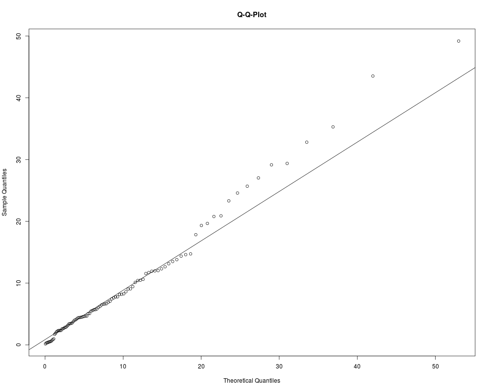
y <- rexp(100, 1/10)
PlotQQ(y, function(p) qexp(p, rate=1/10))

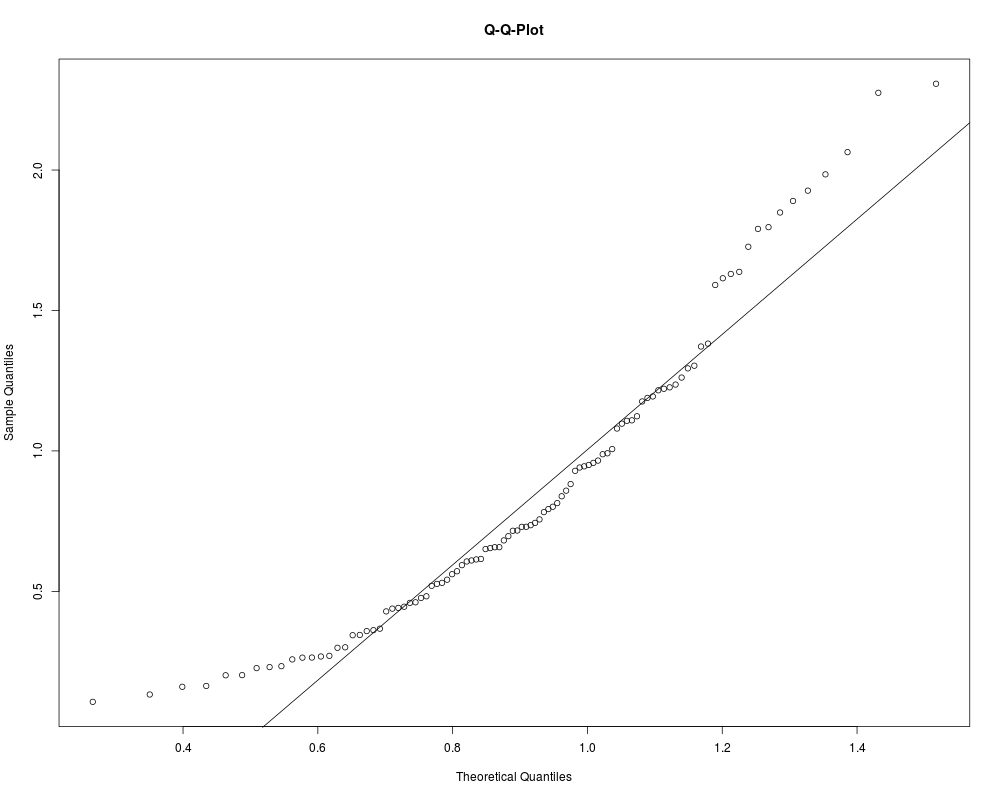
w <- rweibull(100, shape=2)
PlotQQ(w, qdist = function(p) qweibull(p, shape=4))

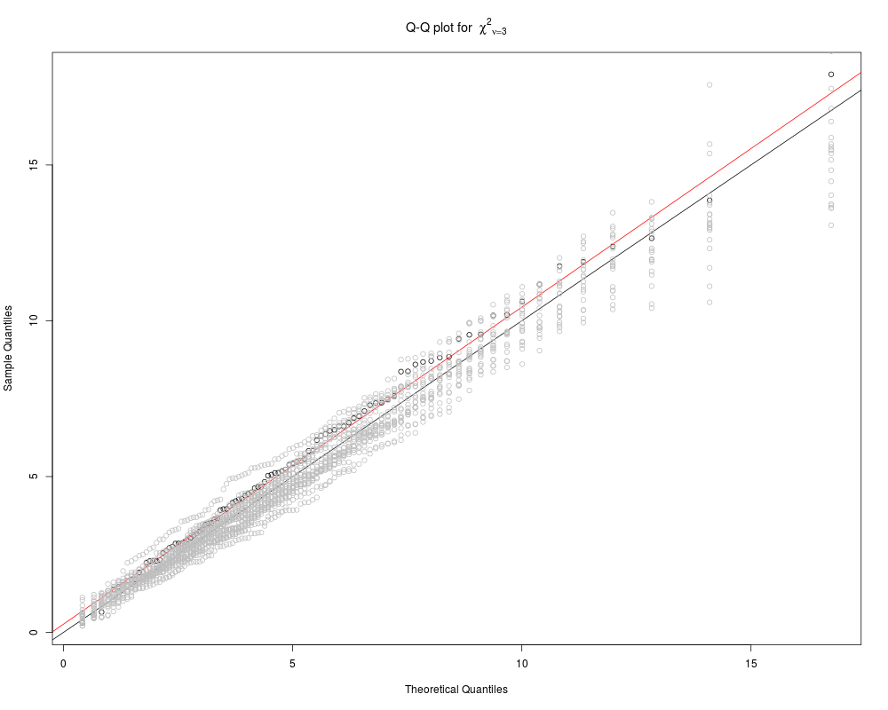
z <- rchisq(100, df=5)
PlotQQ(z, function(p) qchisq(p, df=5), args.qqline=list(col=2, probs=c(0.1,0.6)),
       main=expression("Q-Q plot for" ~~ {chi^2}[nu == 3]))
abline(0,1)

# add 20 random sets
for(i in 1:20){
  z <- rchisq(100, df=5)
  PlotQQ(z, function(p) qchisq(p, df=5), add=TRUE, args.qqline = NA,
         col="grey", lty="dotted")
}

Results


R version 3.3.1 (2016-06-21) -- "Bug in Your Hair"
Copyright (C) 2016 The R Foundation for Statistical Computing
Platform: x86_64-pc-linux-gnu (64-bit)

R is free software and comes with ABSOLUTELY NO WARRANTY.
You are welcome to redistribute it under certain conditions.
Type 'license()' or 'licence()' for distribution details.

R is a collaborative project with many contributors.
Type 'contributors()' for more information and
'citation()' on how to cite R or R packages in publications.

Type 'demo()' for some demos, 'help()' for on-line help, or
'help.start()' for an HTML browser interface to help.
Type 'q()' to quit R.

> library(DescTools)
> png(filename="/home/ddbj/snapshot/RGM3/R_CC/result/DescTools/PlotQQ.Rd_%03d_medium.png", width=480, height=480)
> ### Name: PlotQQ
> ### Title: QQ-Plot for Any Distribution
> ### Aliases: PlotQQ
> ### Keywords: univar hplot
> 
> ### ** Examples
> 
> y <- rexp(100, 1/10)
> PlotQQ(y, function(p) qexp(p, rate=1/10))
> 
> w <- rweibull(100, shape=2)
> PlotQQ(w, qdist = function(p) qweibull(p, shape=4))
> 
> z <- rchisq(100, df=5)
> PlotQQ(z, function(p) qchisq(p, df=5), args.qqline=list(col=2, probs=c(0.1,0.6)),
+        main=expression("Q-Q plot for" ~~ {chi^2}[nu == 3]))
> abline(0,1)
> 
> # add 20 random sets
> for(i in 1:20){
+   z <- rchisq(100, df=5)
+   PlotQQ(z, function(p) qchisq(p, df=5), add=TRUE, args.qqline = NA,
+          col="grey", lty="dotted")
+ }
> 
> 
> 
> 
> 
> dev.off()
null device 
          1 
>