R Graphical Manual

Browse All

Last data update: 2014.03.03

R: Add a Linear Regression Line

lines.lm

R Documentation

Add a Linear Regression Line

Description

Add a linear regression line to an existing plot. The function first calculates the prediction of a lm object for a reasonable amount of points, then adds the line to the plot and inserts a polygon with the confidence and prediction intervals.

Usage

## S3 method for class 'lm'
lines(x, col = getOption("col1", hblue), lwd = 2, lty = "solid", 
        type = "l", n = 100, conf.level = 0.95, args.cband = NULL, 
        pred.level = NA, args.pband = NULL, ...)

Arguments

`x`	linear model object as result from lm(y~x).
`col`	linecolor of the line. Default is DescTools's lightblue.
`lwd`	line width of the line.
`lty`	line type of the line.
`type`	character indicating the type of plotting; actually any of the `types` as in `plot.default`. Type of plot, defaults to `"l"`.
`n`	number of points used for plotting the fit.
`conf.level`	confidence level for the confidence interval. Set this to `NA`, if no confidence band should be plotted. Default is `0.95`.
`args.cband`	list of arguments for the confidence band, such as color or border (see `DrawBand`).
`pred.level`	confidence level for the prediction interval. Set this to NA, if no prediction band should be plotted. Default is `0.95`.
`args.pband`	list of arguments for the prediction band, such as color or border (see `DrawBand`).
`...`	further arguments are not used specifically.

Details

It's sometimes illuminating to plot a regression line with it's prediction, resp. confidence intervals over an existing xy-plot. This only makes sense, if just a simple regression model y ~ x is to be visualized.

Value

nothing

Author(s)

Andri Signorell <andri@signorell.net>

Examples

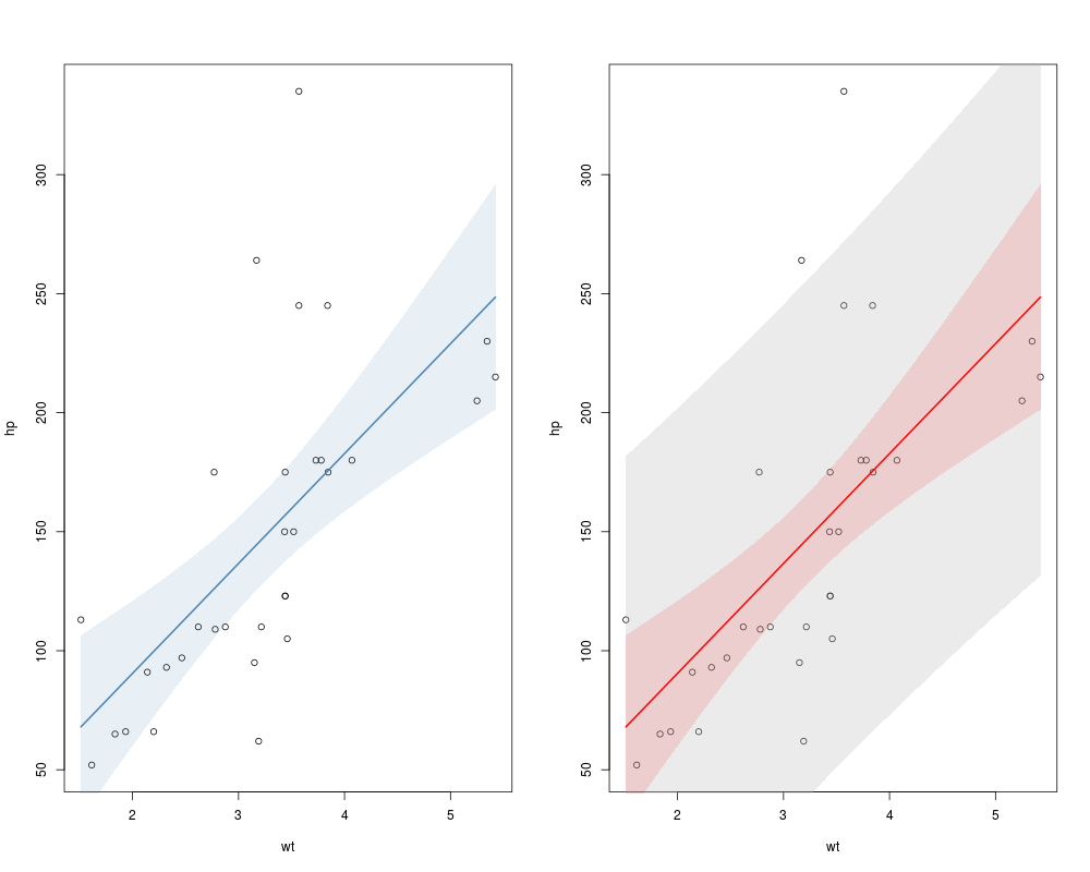
par(mfrow=c(1,2))

plot(hp ~ wt, mtcars)
lines(lm(hp ~ wt, mtcars), col="steelblue")

# add the prediction intervals in different color
plot(hp ~ wt, mtcars)
r.lm <- lm(hp ~ wt, mtcars)
lines(r.lm, col="red", pred.level=0.95, args.pband=list(col=SetAlpha("grey",0.3)) )

Results


R version 3.3.1 (2016-06-21) -- "Bug in Your Hair"
Copyright (C) 2016 The R Foundation for Statistical Computing
Platform: x86_64-pc-linux-gnu (64-bit)

R is free software and comes with ABSOLUTELY NO WARRANTY.
You are welcome to redistribute it under certain conditions.
Type 'license()' or 'licence()' for distribution details.

R is a collaborative project with many contributors.
Type 'contributors()' for more information and
'citation()' on how to cite R or R packages in publications.

Type 'demo()' for some demos, 'help()' for on-line help, or
'help.start()' for an HTML browser interface to help.
Type 'q()' to quit R.

> library(DescTools)
> png(filename="/home/ddbj/snapshot/RGM3/R_CC/result/DescTools/lines.lm.Rd_%03d_medium.png", width=480, height=480)
> ### Name: lines.lm
> ### Title: Add a Linear Regression Line
> ### Aliases: lines.lm
> ### Keywords: aplot math
> 
> ### ** Examples
> 
> par(mfrow=c(1,2))
> 
> plot(hp ~ wt, mtcars)
> lines(lm(hp ~ wt, mtcars), col="steelblue")
> 
> # add the prediction intervals in different color
> plot(hp ~ wt, mtcars)
> r.lm <- lm(hp ~ wt, mtcars)
> lines(r.lm, col="red", pred.level=0.95, args.pband=list(col=SetAlpha("grey",0.3)) )
> 
> 
> 
> 
> 
> dev.off()
null device 
          1 
>