Supported by Dr. Osamu Ogasawara and  . . |
|
Last data update: 2014.03.03 |
Compute the First Passage Time Density of a GQD With Time Inhomogeneous Coefficients.Description
dX_t = (G_0(t)+G_1(t)X_t+G_2(t)X_t^2)dt+√{Q_0(t)+Q_1(t)X_t+Q_2(t)X_t^2}dW_t to a fixed barrier. The function combines the cumulant truncation procedure of Varughese (2013) with a numerical solution to a non-singular Volterra integral equation for the first passage time density, developed by Buonocore et al. (1987), in order to generate an approximate solution. UsageGQD.TIpassage(Xs,B, s, t, delt, theta=c(0), IEQ.type='Buonocore', wrt=FALSE) Arguments
DetailsDetail [1]: First passage throug a time dependant barrier may be analised by applying the transform: Y_t = X_t -B_t, if B_t may can be decomposed as B_t = k+f(t). By applying Ito's lemma the revised drift and diffusion functionals, and first passage parameters may be inferred. Detail [2]: The starting time is of particular importance when the drift and/or diffusion terms are time-inhomogeneous. Take care to select the correct starting time - especially if the drift or diffusion components whch are time dependant have poles or singular points in the time domain. Value
WarningWarning [1]: Some instability may occur when Warning [2]:The first passage time problem is considered from one side only i.e. Xs<B. For Xs>B one may equivalently consider Yt=-X_t, apply Ito's lemma and proceed as above. NoteNote [1]: The coefficients od the GQD may be parameterized using the reserved variable
may be used so long as values are asigned in the function call, say
Note [2]: Due to syntactical differences between R and C++ special functions have to be used when terms that depend on
Here sqrt(t)*cos(3*pi*t) constitutes the product of two terms that cannot be written i.t.o. a single Note [3]: Similarly, the ^ - operator is not overloaded in C++. Instead the
Note [4]: Author(s)Etienne A.D. Pienaar: etiennead@gmail.com ReferencesUpdates available on GitHub at https://github.com/eta21. A. Buonocore, A. Nobile, and L. Ricciardi. 1987 A new integral equation for the evaluation of first-passage- time probability densities. Adv. Appl. Probab. 19:784–800. Daniels, H.E. 1954 Saddlepoint approximations in statistics. Ann. Math. Stat., 25:631–650. Eddelbuettel, D. and Romain, F. 2011 Rcpp: Seamless R and C++ integration. Journal of Statistical Software, 40(8):1–18,. URL http://www.jstatsoft.org/v40/i08/. Eddelbuettel, D. 2013 Seamless R and C++ Integration with Rcpp. New York: Springer. ISBN 978-1-4614-6867-7. Eddelbuettel, D. and Sanderson, C. 2014 Rcpparmadillo: Accelerating r with high-performance C++ linear algebra. Computational Statistics and Data Analysis, 71:1054–1063. URL http://dx.doi.org/10.1016/j.csda.2013.02.005. Feagin, T. 2007 A tenth-order Runge-Kutta method with error estimate. In Proceedings of the IAENG Conf. on Scientific Computing. R. G. Jaimez, P. R. Roman and F. T. Ruiz. 1995 A note on the volterra integral equation for the first-passage-time probability density. Journal of applied probability, 635–648. Varughese, M.M. 2013 Parameter estimation for multivariate diffusion systems. Comput. Stat. Data An., 57:417–428. See Also
Examples
#=========================================================================
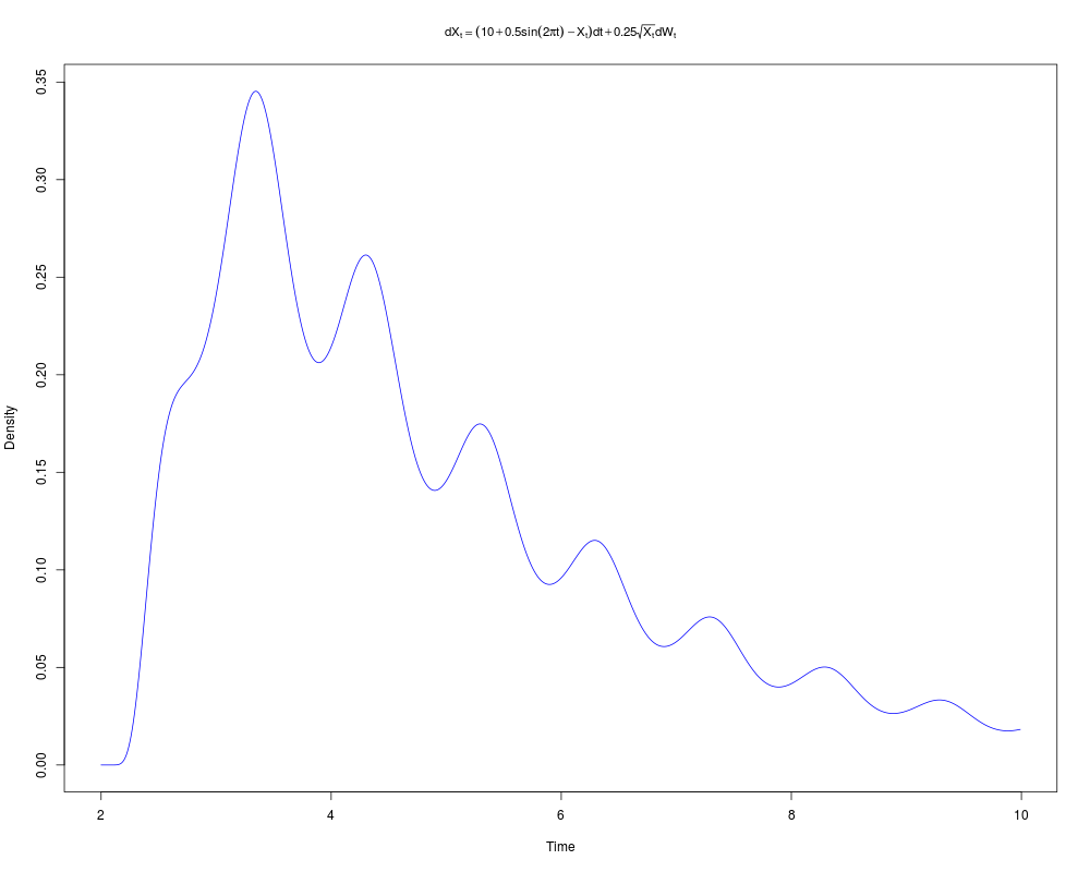
# Generate the first passage time density of a CIR process with time
# dependant drift to a fixed barrier.
#-------------------------------------------------------------------------
# Remove any existing coefficients.
GQD.remove()
# Define the coefficients of the process.
G0 <- function(t){10+0.5*sin(2*pi*t)}
G1 <- function(t){-1}
Q1 <- function(t){0.25}
#Define the parameters of the first passage time problem.
delt <- 1/100 # The stepsize for the solution
X0 <- 8 # The initial value of the process
BB <- 11 # Fixed barrier
T0 <- 2 # Starting time of the diffusion
TT <- 10 # Time horizon of the computation
# Run the calculation
res1 <- GQD.TIpassage(X0,BB,T0,TT,delt)
# Remove any existing coefficients.
GQD.remove()
# Redefine the coefficients.
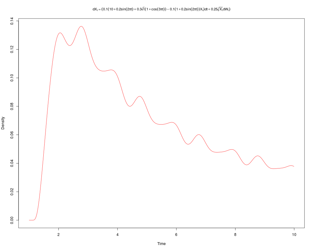
G0 <- function(t){ 0.1*(10+0.2*sin(2*pi*t)+0.3*prod(sqrt(t),1+cos(3*pi*t)))}
G1 <- function(t){-0.1*(1+0.2*sin(2*pi*t))}
Q1 <- function(t){0.25}
# Redefine the parameters of the f.p.t. problem.
delt <- 1/100
X0 <- 8
BB <- 11
T0 <- 1
TT <- 10
# Run the calculation
res2 <- GQD.TIpassage(X0,BB,T0,TT,delt)
#===============================================================================
# Plot the two solutions.
#===============================================================================
expr1 <- expression(dX[t]==(10+0.5*sin(2*pi*t)-X[t])*dt+0.25*sqrt(X[t])*dW[t])
expr2 <- expression(dX[t]==(0.1*(10+0.2*sin(2*pi*t)+0.3*sqrt(t)*(1+cos(3*pi*t))
-0.1*(1+0.2*sin(2*pi*t))*X[t])*dt+0.25*sqrt(X[t])*dW[t]))
par(mfrow=c(1,1))
plot(res1$density~res1$time,type='l',col='blue',
ylab='Density',xlab='Time',main=expr1,cex.main=0.95)
plot(res2$density~res2$time,type='l',col='red',
ylab='Density',xlab='Time',main =expr2,cex.main=0.95)
#===============================================================================
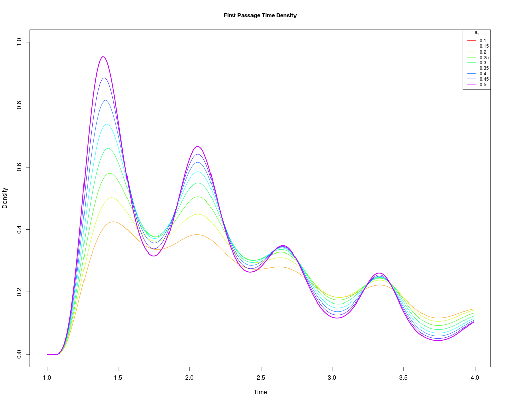
# Let's see how sensitive the first passage density is w.r.t a speed parameter
# of a non-linear diffusion.
#===============================================================================
GQD.remove()
# Redefine the coefficients with a parameter theta:
G1 <- function(t){theta[1]*(10+0.2*sin(2*pi*t)+0.3*prod(sqrt(t),1+cos(3*pi*t)))}
G2 <- function(t){-theta[1]}
Q2 <- function(t){0.1}
# Now just give a value for the parameter in the standard fashion:
res3=GQD.TIpassage(8,12,1,4,1/100,theta=c(0.5))
plot(res3$density~res3$time,type='l',col=2,ylim=c(0,1.0),
main='First Passage Time Density',ylab='Density',xlab='Time',cex.main=0.95)
# Change the parameter and see the effect on the f.p.t. density.
th.seq=seq(0.1,0.5,1/20)
for(i in 2:length(th.seq))
{
res3=GQD.TIpassage(8,12,1,4,1/100,,theta=c(th.seq[i]))
lines(res3$density~res3$time,type='l',col=rainbow(10)[i])
}
lines(res3$density~res3$time,type='l',col=rainbow(10)[i],lwd=2)
legend('topright',legend=th.seq,col=rainbow(10),lty='solid',cex=0.75,
title=expression(theta[1]))
#===============================================================================
Results
R version 3.3.1 (2016-06-21) -- "Bug in Your Hair"
Copyright (C) 2016 The R Foundation for Statistical Computing
Platform: x86_64-pc-linux-gnu (64-bit)

R is free software and comes with ABSOLUTELY NO WARRANTY.
You are welcome to redistribute it under certain conditions.
Type 'license()' or 'licence()' for distribution details.

R is a collaborative project with many contributors.
Type 'contributors()' for more information and
'citation()' on how to cite R or R packages in publications.

Type 'demo()' for some demos, 'help()' for on-line help, or
'help.start()' for an HTML browser interface to help.
Type 'q()' to quit R.

> library(DiffusionRgqd)
> png(filename="/home/ddbj/snapshot/RGM3/R_CC/result/DiffusionRgqd/GQD.TIpassage.Rd_%03d_medium.png", width=480, height=480)
> ### Name: GQD.TIpassage
> ### Title: Compute the First Passage Time Density of a GQD With Time
> ###   Inhomogeneous Coefficients.
> ### Aliases: GQD.TIpassage
> ### Keywords: syntax C++ first passage time
>
> ### ** Examples
>
> ## No test:
> #=========================================================================
> # Generate the first passage time density of a CIR process with time
> # dependant drift to a fixed barrier.
> #-------------------------------------------------------------------------
>
>   # Remove any existing coefficients.
>   GQD.remove()
[1] "Removed :  NA "
>
>   # Define the coefficients of the process.
>   G0 <- function(t){10+0.5*sin(2*pi*t)}
>   G1 <- function(t){-1}
>   Q1 <- function(t){0.25}
>
>
>   #Define the parameters of the first passage time problem.
>   delt  <- 1/100         # The stepsize for the solution
>   X0 <- 8                # The initial value of the process
>   BB <- 11               # Fixed barrier
>   T0 <- 2                # Starting time of the diffusion
>   TT <- 10                # Time horizon of the computation
>
>   # Run the calculation
>   res1 <- GQD.TIpassage(X0,BB,T0,TT,delt)
Compiling C++ code. Please wait.                                          >
>   # Remove any existing coefficients.
>   GQD.remove()
[1] "Removed :  G0 G1 Q1"
>
>   # Redefine the coefficients.
>   G0 <- function(t){ 0.1*(10+0.2*sin(2*pi*t)+0.3*prod(sqrt(t),1+cos(3*pi*t)))}
>   G1 <- function(t){-0.1*(1+0.2*sin(2*pi*t))}
>   Q1 <- function(t){0.25}
>
>   # Redefine the parameters of the f.p.t. problem.
>
>   delt  <- 1/100
>   X0 <- 8
>   BB <- 11
>   T0 <- 1
>   TT <- 10
>
>   # Run the calculation
>   res2 <- GQD.TIpassage(X0,BB,T0,TT,delt)
Compiling C++ code. Please wait.                                          >
> #===============================================================================
> # Plot the two solutions.
> #===============================================================================
>   expr1 <- expression(dX[t]==(10+0.5*sin(2*pi*t)-X[t])*dt+0.25*sqrt(X[t])*dW[t])
>   expr2 <- expression(dX[t]==(0.1*(10+0.2*sin(2*pi*t)+0.3*sqrt(t)*(1+cos(3*pi*t))
+                       -0.1*(1+0.2*sin(2*pi*t))*X[t])*dt+0.25*sqrt(X[t])*dW[t]))
>
>
>   par(mfrow=c(1,1))
>   plot(res1$density~res1$time,type='l',col='blue',
+        ylab='Density',xlab='Time',main=expr1,cex.main=0.95)
>
>   plot(res2$density~res2$time,type='l',col='red',
+        ylab='Density',xlab='Time',main =expr2,cex.main=0.95)
>
> #===============================================================================
> # Let's see how sensitive the first passage density is w.r.t a speed parameter
> # of a non-linear diffusion.
> #===============================================================================
>
> GQD.remove()
[1] "Removed :  G0 G1 Q1"
> # Redefine the coefficients with a parameter theta:
> G1 <- function(t){theta[1]*(10+0.2*sin(2*pi*t)+0.3*prod(sqrt(t),1+cos(3*pi*t)))}
> G2 <- function(t){-theta[1]}
> Q2 <- function(t){0.1}
> # Now just give a value for the parameter in the standard fashion:
> res3=GQD.TIpassage(8,12,1,4,1/100,theta=c(0.5))
Compiling C++ code. Please wait.                                          >
> plot(res3$density~res3$time,type='l',col=2,ylim=c(0,1.0),
+ main='First Passage Time Density',ylab='Density',xlab='Time',cex.main=0.95)
> # Change the parameter and see the effect on the f.p.t. density.
> th.seq=seq(0.1,0.5,1/20)
> for(i in 2:length(th.seq))
+ {
+   res3=GQD.TIpassage(8,12,1,4,1/100,,theta=c(th.seq[i]))
+   lines(res3$density~res3$time,type='l',col=rainbow(10)[i])
+ }
Compiling C++ code. Please wait.                                          Compiling C++ code. Please wait.                                          Compiling C++ code. Please wait.                                          Compiling C++ code. Please wait.                                          Compiling C++ code. Please wait.                                          Compiling C++ code. Please wait.                                          Compiling C++ code. Please wait.                                          Compiling C++ code. Please wait.                                          > lines(res3$density~res3$time,type='l',col=rainbow(10)[i],lwd=2)
> legend('topright',legend=th.seq,col=rainbow(10),lty='solid',cex=0.75,
+ title=expression(theta[1]))
> #===============================================================================
> ## End(No test)
>
>
>
>
>
> dev.off()
null device
          1
>
|