revised MLearn interface for machine learning

Description

revised MLearn interface for machine learning, emphasizing a schematic description of external learning functions like knn, lda, nnet, etc.

Usage

MLearn( formula, data, .method, trainInd, ... )
makeLearnerSchema(packname, mlfunname, converter, predicter)

Arguments

Details

The purpose of the MLearn methods is to provide a uniform calling sequence to diverse machine learning algorithms. In R package, machine learning functions can have parameters (x, y, ...) or (formula, data, ...) or some other sequence, and these functions can return lists or vectors or other sorts of things. With MLearn, we always have calling sequence MLearn(formula, data, .method, trainInd, ...), and data can be a data.frame or ExpressionSet. MLearn will always return an S4 instance of classifierObject or clusteringObject.

At this time (1.13.x), NA values in predictors trigger an error.

To obtain documentation on the older (pre bioc 2.1) version of the MLearn method, please use help(MLearn-OLD).

randomForestI

randomForest. Note, that to obtain the default performance of randomForestB, you need to set mtry and sampsize parameters to sqrt(number of features) and table([training set response factor]) respectively, as these were not taken to be the function's defaults. Note you can use xvalSpec("NOTEST") as trainInd, to use all the samples; the RObject() result will print the misclassification matrix estimate along with OOB error rate estimate.

knnI(k=1,l=0)

knn; special support bridge required, defined in MLint

knn.cvI(k=1,l=0)

knn.cv; special support bridge required, defined in MLint. This option uses the embedded leave-one-out cross-validation of knn.cv, and thereby achieves high performance. You can have more general cross-validation using knnI with an xvalSpec, but it will be slower. When using this learner schema, you should use the numerical trainInd setting with 1:N where N is the number of samples.

dldaI

diagDA; special support bridge required, defined in MLint

nnetI

nnet

rpartI

rpart

ldaI

lda

svmI

svm

qdaI

qda

logisticI(threshold)

glm – with binomial family, expecting a dichotomous factor as response variable, not bulletproofed against other responses yet. If response probability estimate exceeds threshold, predict 1, else 0

adaI

ada

BgbmI

gbm, forcing the Bernoulli loss function.

blackboostI

blackboost – you MUST supply a family parameter relevant for mboost package procedures

lvqI

lvqtest after building codebook with lvqinit and updating with olvq1. You will need to write your own detailed schema if you want to tweak tuning parameters.

naiveBayesI

naiveBayes

baggingI

bagging

sldaI

slda

rdaI

rda – you must supply the alpha and delta parameters to use this. Typically cross-validation is used to select these. See rdacvI below.

rdacvI

rda.cv. This interface is complicated. The typical use includes cross-validation internal to the rda.cv function. That process searches a tuning parameter space and delivers an ordering on parameters. The interface selects the parameters by looking at all parameter configurations achieving the smallest min+1SE cv.error estimate, and taking the one among them that employed the -most- features (agnosticism). A final run of rda is then conducted with the tuning parameters set at that 'optimal' choice. The bridge code can be modified to facilitate alternative choices of the parameters in use. plotXvalRDA is an interface to the plot method for objects of class rdacv defined in package rda. You can use xvalSpec("NOTEST") with this procedure to use all the samples to build the discriminator.

ksvmI

ksvm

hclustI(distMethod, agglomMethod)

hclust – you must explicitly specify distance and agglomeration procedure.

kmeansI(centers, algorithm)

kmeans – you must explicitly specify centers and algorithm name.

If the parallel package is attached, cross-validation will be distributed to cores using mclapply.

Value

Instances of classifierOutput or clusteringOutput

Author(s)

Vince Carey <stvjc@channing.harvard.edu>

See Also

Try example(hclustWidget, ask=FALSE) for an interactive approach to cluster analysis tuning.

Examples

library("MASS")
data(crabs)
set.seed(1234)
kp = sample(1:200, size=120)
rf1 = MLearn(sp~CW+RW, data=crabs, randomForestI, kp, ntree=600 )
rf1
nn1 = MLearn(sp~CW+RW, data=crabs, nnetI, kp, size=3, decay=.01,
    trace=FALSE )
nn1
RObject(nn1)
knn1 = MLearn(sp~CW+RW, data=crabs, knnI(k=3,l=2), kp)
knn1
names(RObject(knn1))
dlda1 = MLearn(sp~CW+RW, data=crabs, dldaI, kp )
dlda1
names(RObject(dlda1))
lda1 = MLearn(sp~CW+RW, data=crabs, ldaI, kp )
lda1
names(RObject(lda1))
slda1 = MLearn(sp~CW+RW, data=crabs, sldaI, kp )
slda1
names(RObject(slda1))
svm1 = MLearn(sp~CW+RW, data=crabs, svmI, kp )
svm1
names(RObject(svm1))
ldapp1 = MLearn(sp~CW+RW, data=crabs, ldaI.predParms(method="debiased"), kp )
ldapp1
names(RObject(ldapp1))
qda1 = MLearn(sp~CW+RW, data=crabs, qdaI, kp )
qda1
names(RObject(qda1))
logi = MLearn(sp~CW+RW, data=crabs, glmI.logistic(threshold=0.5), kp, family=binomial ) # need family
logi
names(RObject(logi))
rp2 = MLearn(sp~CW+RW, data=crabs, rpartI, kp)
rp2
## recode data for RAB
#nsp = ifelse(crabs$sp=="O", -1, 1)
#nsp = factor(nsp)
#ncrabs = cbind(nsp,crabs)
#rab1 = MLearn(nsp~CW+RW, data=ncrabs, RABI, kp, maxiter=10)
#rab1
#
# new approach to adaboost
#
ada1 = MLearn(sp ~ CW+RW, data = crabs, .method = adaI, 
    trainInd = kp, type = "discrete", iter = 200)
ada1
confuMat(ada1)
#
lvq.1 = MLearn(sp~CW+RW, data=crabs, lvqI, kp )
lvq.1
nb.1 = MLearn(sp~CW+RW, data=crabs, naiveBayesI, kp )
confuMat(nb.1)
bb.1 = MLearn(sp~CW+RW, data=crabs, baggingI, kp )
confuMat(bb.1)
#
# new mboost interface -- you MUST supply family for nonGaussian response
#
require(party)  # trafo ... killing cmd check
blb.1 = MLearn(sp~CW+RW+FL, data=crabs, blackboostI, kp, family=mboost::Binomial() )
confuMat(blb.1)
#
# ExpressionSet illustration
# 
data(sample.ExpressionSet)
#  needed to increase training set size to avoid a new randomForest condition
# on empty class
set.seed(1234)
X = MLearn(type~., sample.ExpressionSet[100:250,], randomForestI, 1:19, importance=TRUE )
library(randomForest)
library(hgu95av2.db)
opar = par(no.readonly=TRUE)
par(las=2)
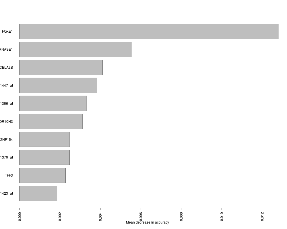
plot(getVarImp(X), n=10, plat="hgu95av2", toktype="SYMBOL")
par(opar)
#
# demonstrate cross validation
#
nn1cv = MLearn(sp~CW+RW, data=crabs[c(1:20,101:120),], 
   nnetI, xvalSpec("LOO"), size=3, decay=.01, trace=FALSE )
confuMat(nn1cv)
nn2cv = MLearn(sp~CW+RW, data=crabs[c(1:20,101:120),], nnetI, 
   xvalSpec("LOG",5, balKfold.xvspec(5)), size=3, decay=.01,
   trace=FALSE )
confuMat(nn2cv)
nn3cv = MLearn(sp~CW+RW+CL+BD+FL, data=crabs[c(1:20,101:120),], nnetI, 
   xvalSpec("LOG",5, balKfold.xvspec(5), fsFun=fs.absT(2)), size=3, decay=.01,
   trace=FALSE )
confuMat(nn3cv)
nn4cv = MLearn(sp~.-index-sex, data=crabs[c(1:20,101:120),], nnetI, 
   xvalSpec("LOG",5, balKfold.xvspec(5), fsFun=fs.absT(2)), size=3, decay=.01,
   trace=FALSE )
confuMat(nn4cv)
#
# try with expression data
#
library(golubEsets)
data(Golub_Train)
litg = Golub_Train[ 100:150, ]
g1 = MLearn(ALL.AML~. , litg, nnetI, 
   xvalSpec("LOG",5, balKfold.xvspec(5), 
   fsFun=fs.probT(.75)), size=3, decay=.01, trace=FALSE )
confuMat(g1)
#
# illustrate rda.cv interface from package rda (requiring local bridge)
#
library(ALL)
data(ALL)
#
# restrict to BCR/ABL or NEG
#
bio <- which( ALL$mol.biol %in% c("BCR/ABL", "NEG"))
#
# restrict to B-cell
#
isb <- grep("^B", as.character(ALL$BT))
kp <- intersect(bio,isb)
all2 <- ALL[,kp]
mads = apply(exprs(all2),1,mad)
kp = which(mads>1)  # get around 250 genes
vall2 = all2[kp, ]
vall2$mol.biol = factor(vall2$mol.biol) # drop unused levels

r1 = MLearn(mol.biol~., vall2, rdacvI, 1:40)
confuMat(r1)
RObject(r1)
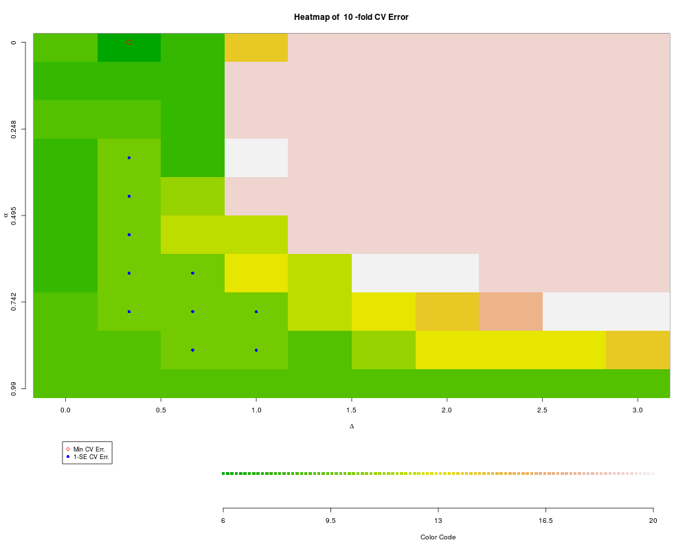
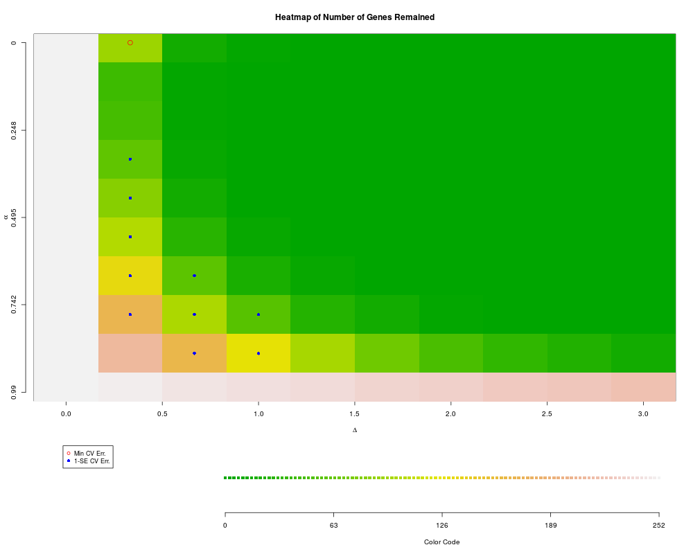
plotXvalRDA(r1)  # special interface to plots of parameter space

# illustrate clustering support

cl1 = MLearn(~CW+RW+CL+FL+BD, data=crabs, hclustI(distFun=dist, cutParm=list(k=4)))
plot(cl1)

cl1a = MLearn(~CW+RW+CL+FL+BD, data=crabs, hclustI(distFun=dist, cutParm=list(k=4)), 
   method="complete")
plot(cl1a)

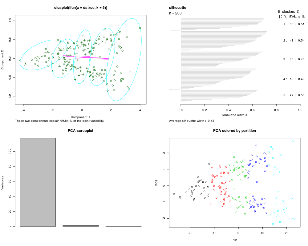
cl2 = MLearn(~CW+RW+CL+FL+BD, data=crabs, kmeansI, centers=5, algorithm="Hartigan-Wong")
plot(cl2, crabs[,-c(1:3)])

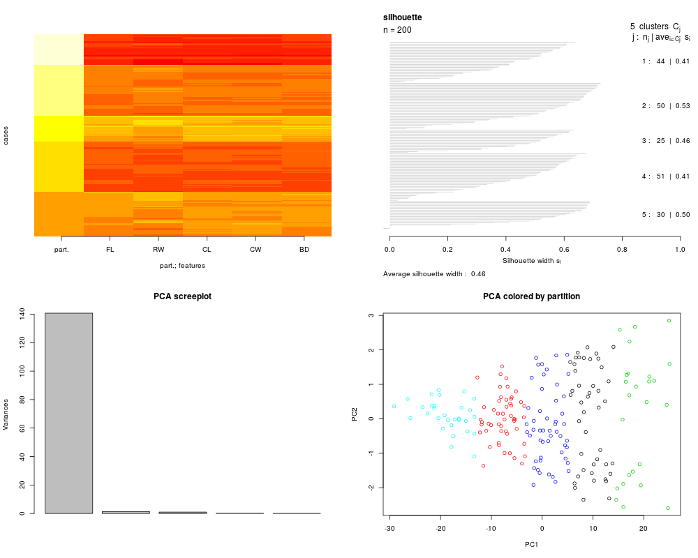
c3 = MLearn(~CL+CW+RW, crabs, pamI(dist), k=5)
c3
plot(c3, data=crabs[,c("CL", "CW", "RW")])


#  new interfaces to PLS thanks to Laurent Gatto

set.seed(1234)
kp = sample(1:200, size=120)

plsda.1 = MLearn(sp~CW+RW, data=crabs, plsdaI, kp, probMethod="Bayes")
plsda.1
confuMat(plsda.1)
confuMat(plsda.1,t=.65) ## requires at least 0.65 post error prob to assign species

plsda.2 = MLearn(type~., data=sample.ExpressionSet[100:250,], plsdaI, 1:16)
plsda.2
confuMat(plsda.2)
confuMat(plsda.2,t=.65) ## requires at least 0.65 post error prob to assign outcome

## examples for predict
clout <- MLearn(type~., sample.ExpressionSet[100:250,], svmI , 1:16)
predict(clout, sample.ExpressionSet[100:250,17:26])

Results

R version 3.3.1 (2016-06-21) -- "Bug in Your Hair"
Copyright (C) 2016 The R Foundation for Statistical Computing
Platform: x86_64-pc-linux-gnu (64-bit)

R is free software and comes with ABSOLUTELY NO WARRANTY.
You are welcome to redistribute it under certain conditions.
Type 'license()' or 'licence()' for distribution details.

R is a collaborative project with many contributors.
Type 'contributors()' for more information and
'citation()' on how to cite R or R packages in publications.

Type 'demo()' for some demos, 'help()' for on-line help, or
'help.start()' for an HTML browser interface to help.
Type 'q()' to quit R.

> library(MLInterfaces)
Loading required package: BiocGenerics
Loading required package: parallel

Attaching package: 'BiocGenerics'

The following objects are masked from 'package:parallel':

    clusterApply, clusterApplyLB, clusterCall, clusterEvalQ,
    clusterExport, clusterMap, parApply, parCapply, parLapply,
    parLapplyLB, parRapply, parSapply, parSapplyLB

The following objects are masked from 'package:stats':

    IQR, mad, xtabs

The following objects are masked from 'package:base':

    Filter, Find, Map, Position, Reduce, anyDuplicated, append,
    as.data.frame, cbind, colnames, do.call, duplicated, eval, evalq,
    get, grep, grepl, intersect, is.unsorted, lapply, lengths, mapply,
    match, mget, order, paste, pmax, pmax.int, pmin, pmin.int, rank,
    rbind, rownames, sapply, setdiff, sort, table, tapply, union,
    unique, unsplit

Loading required package: Biobase
Welcome to Bioconductor

    Vignettes contain introductory material; view with
    'browseVignettes()'. To cite Bioconductor, see
    'citation("Biobase")', and for packages 'citation("pkgname")'.

Loading required package: annotate
Loading required package: AnnotationDbi
Loading required package: stats4
Loading required package: IRanges
Loading required package: S4Vectors

Attaching package: 'S4Vectors'

The following objects are masked from 'package:base':

    colMeans, colSums, expand.grid, rowMeans, rowSums

Loading required package: XML
Loading required package: cluster
> png(filename="/home/ddbj/snapshot/RGM3/R_BC/result/MLInterfaces/MLearn-new.Rd_%03d_medium.png", width=480, height=480)
> ### Name: MLearn
> ### Title: revised MLearn interface for machine learning
> ### Aliases: MLearn_new MLearn baggingI dlda glmI.logistic knnI knn.cvI
> ###   ksvmI ldaI lvqI naiveBayesI nnetI qdaI RABI randomForestI rpartI svmI
> ###   svm2 ksvm2 plsda2 plsdaI dlda2 dldaI sldaI blackboostI knn2 knn.cv2
> ###   ldaI.predParms lvq rab adaI
> ###   MLearn,formula,ExpressionSet,character,numeric-method
> ###   MLearn,formula,ExpressionSet,learnerSchema,numeric-method
> ###   MLearn,formula,data.frame,learnerSchema,numeric-method
> ###   MLearn,formula,data.frame,learnerSchema,xvalSpec-method
> ###   MLearn,formula,ExpressionSet,learnerSchema,xvalSpec-method
> ###   MLearn,formula,data.frame,clusteringSchema,ANY-method plotXvalRDA
> ###   rdacvI rdaI BgbmI gbm2 rdaML rdacvML hclustI kmeansI pamI
> ###   makeLearnerSchema standardMLIConverter
> ### Keywords: models
> 
> ### ** Examples
> 
> library("MASS")

Attaching package: 'MASS'

The following object is masked from 'package:AnnotationDbi':

    select

> data(crabs)
> set.seed(1234)
> kp = sample(1:200, size=120)
> rf1 = MLearn(sp~CW+RW, data=crabs, randomForestI, kp, ntree=600 )
> rf1
MLInterfaces classification output container
The call was:
MLearn(formula = sp ~ CW + RW, data = crabs, .method = randomForestI, 
    trainInd = kp, ntree = 600)
Predicted outcome distribution for test set:

 B  O 
42 38 
Summary of scores on test set (use testScores() method for details):
        B         O 
0.5265625 0.4734375 
> nn1 = MLearn(sp~CW+RW, data=crabs, nnetI, kp, size=3, decay=.01,
+     trace=FALSE )
> nn1
MLInterfaces classification output container
The call was:
MLearn(formula = sp ~ CW + RW, data = crabs, .method = nnetI, 
    trainInd = kp, size = 3, decay = 0.01, trace = FALSE)
Predicted outcome distribution for test set:

 B  O 
21 59 
Summary of scores on test set (use testScores() method for details):
[1] 0.5182391
> RObject(nn1)
a 2-3-1 network with 13 weights
inputs: CW RW 
output(s): sp 
options were - entropy fitting  decay=0.01
> knn1 = MLearn(sp~CW+RW, data=crabs, knnI(k=3,l=2), kp)
> knn1
MLInterfaces classification output container
The call was:
MLearn(formula = sp ~ CW + RW, data = crabs, .method = knnI(k = 3, 
    l = 2), trainInd = kp)
Predicted outcome distribution for test set:

 B  O 
44 36 
Summary of scores on test set (use testScores() method for details):
   Min. 1st Qu.  Median    Mean 3rd Qu.    Max. 
 0.5000  0.6667  0.6667  0.7552  1.0000  1.0000 
> names(RObject(knn1))
[1] "traindat" "ans"      "traincl" 
> dlda1 = MLearn(sp~CW+RW, data=crabs, dldaI, kp )
> dlda1
MLInterfaces classification output container
The call was:
MLearn(formula = sp ~ CW + RW, data = crabs, .method = dldaI, 
    trainInd = kp)
Predicted outcome distribution for test set:

 B  O 
40 40 
> names(RObject(dlda1))
[1] "traindat" "ans"      "traincl" 
> lda1 = MLearn(sp~CW+RW, data=crabs, ldaI, kp )
> lda1
MLInterfaces classification output container
The call was:
MLearn(formula = sp ~ CW + RW, data = crabs, .method = ldaI, 
    trainInd = kp)
Predicted outcome distribution for test set:

 B  O 
43 37 
> names(RObject(lda1))
 [1] "prior"   "counts"  "means"   "scaling" "lev"     "svd"     "N"      
 [8] "call"    "terms"   "xlevels"
> slda1 = MLearn(sp~CW+RW, data=crabs, sldaI, kp )
> slda1
MLInterfaces classification output container
The call was:
MLearn(formula = sp ~ CW + RW, data = crabs, .method = sldaI, 
    trainInd = kp)
Predicted outcome distribution for test set:

 B  O 
49 31 
Summary of scores on test set (use testScores() method for details):
       B        O 
0.539828 0.460172 
> names(RObject(slda1))
[1] "scores"  "mylda"   "terms"   "call"    "xlevels"
> svm1 = MLearn(sp~CW+RW, data=crabs, svmI, kp )
> svm1
MLInterfaces classification output container
The call was:
MLearn(formula = sp ~ CW + RW, data = crabs, .method = svmI, 
    trainInd = kp)
Predicted outcome distribution for test set:

 B  O 
49 31 
Summary of scores on test set (use testScores() method for details):
        B         O 
0.5139337 0.4860663 
> names(RObject(svm1))
 [1] "call"            "type"            "kernel"          "cost"           
 [5] "degree"          "gamma"           "coef0"           "nu"             
 [9] "epsilon"         "sparse"          "scaled"          "x.scale"        
[13] "y.scale"         "nclasses"        "levels"          "tot.nSV"        
[17] "nSV"             "labels"          "SV"              "index"          
[21] "rho"             "compprob"        "probA"           "probB"          
[25] "sigma"           "coefs"           "na.action"       "fitted"         
[29] "decision.values" "terms"          
> ldapp1 = MLearn(sp~CW+RW, data=crabs, ldaI.predParms(method="debiased"), kp )
> ldapp1
MLInterfaces classification output container
The call was:
MLearn(formula = sp ~ CW + RW, data = crabs, .method = ldaI.predParms(method = "debiased"), 
    trainInd = kp)
Predicted outcome distribution for test set:

 B  O 
43 37 
> names(RObject(ldapp1))
 [1] "prior"   "counts"  "means"   "scaling" "lev"     "svd"     "N"      
 [8] "call"    "terms"   "xlevels"
> qda1 = MLearn(sp~CW+RW, data=crabs, qdaI, kp )
> qda1
MLInterfaces classification output container
The call was:
MLearn(formula = sp ~ CW + RW, data = crabs, .method = qdaI, 
    trainInd = kp)
Predicted outcome distribution for test set:

 B  O 
47 33 
> names(RObject(qda1))
 [1] "prior"   "counts"  "means"   "scaling" "ldet"    "lev"     "N"      
 [8] "call"    "terms"   "xlevels"
> logi = MLearn(sp~CW+RW, data=crabs, glmI.logistic(threshold=0.5), kp, family=binomial ) # need family
> logi
MLInterfaces classification output container
The call was:
MLearn(formula = sp ~ CW + RW, data = crabs, .method = glmI.logistic(threshold = 0.5), 
    trainInd = kp, family = binomial)
Predicted outcome distribution for test set:

 B  O 
42 38 
Summary of scores on test set (use testScores() method for details):
   Min. 1st Qu.  Median    Mean 3rd Qu.    Max. 
 0.1621  0.3617  0.4868  0.5175  0.6751  0.8831 
> names(RObject(logi))
 [1] "coefficients"      "residuals"         "fitted.values"    
 [4] "effects"           "R"                 "rank"             
 [7] "qr"                "family"            "linear.predictors"
[10] "deviance"          "aic"               "null.deviance"    
[13] "iter"              "weights"           "prior.weights"    
[16] "df.residual"       "df.null"           "y"                
[19] "converged"         "boundary"          "model"            
[22] "call"              "formula"           "terms"            
[25] "data"              "offset"            "control"          
[28] "method"            "contrasts"         "xlevels"          
> rp2 = MLearn(sp~CW+RW, data=crabs, rpartI, kp)
> rp2
MLInterfaces classification output container
The call was:
MLearn(formula = sp ~ CW + RW, data = crabs, .method = rpartI, 
    trainInd = kp)
Predicted outcome distribution for test set:

 B  O 
50 30 
Summary of scores on test set (use testScores() method for details):
        B         O 
0.5619216 0.4380784 
> ## recode data for RAB
> #nsp = ifelse(crabs$sp=="O", -1, 1)
> #nsp = factor(nsp)
> #ncrabs = cbind(nsp,crabs)
> #rab1 = MLearn(nsp~CW+RW, data=ncrabs, RABI, kp, maxiter=10)
> #rab1
> #
> # new approach to adaboost
> #
> ada1 = MLearn(sp ~ CW+RW, data = crabs, .method = adaI, 
+     trainInd = kp, type = "discrete", iter = 200)
> ada1
MLInterfaces classification output container
The call was:
MLearn(formula = sp ~ CW + RW, data = crabs, .method = adaI, 
    trainInd = kp, type = "discrete", iter = 200)
Predicted outcome distribution for test set:

 B  O 
47 33 
> confuMat(ada1)
     predicted
given  B  O
    B 25 12
    O 22 21
> #
> lvq.1 = MLearn(sp~CW+RW, data=crabs, lvqI, kp )
> lvq.1
MLInterfaces classification output container
The call was:
MLearn(formula = sp ~ CW + RW, data = crabs, .method = lvqI, 
    trainInd = kp)
Predicted outcome distribution for test set:

 B  O 
38 42 
> nb.1 = MLearn(sp~CW+RW, data=crabs, naiveBayesI, kp )
> confuMat(nb.1)
     predicted
given  B  O
    B 25 12
    O 17 26
> bb.1 = MLearn(sp~CW+RW, data=crabs, baggingI, kp )
> confuMat(bb.1)
     predicted
given  B  O
    B 20 17
    O 22 21
> #
> # new mboost interface -- you MUST supply family for nonGaussian response
> #
> require(party)  # trafo ... killing cmd check
Loading required package: party
Loading required package: grid
Loading required package: mvtnorm
Loading required package: modeltools

Attaching package: 'modeltools'

The following object is masked from 'package:MLInterfaces':

    Predict

Loading required package: strucchange
Loading required package: zoo

Attaching package: 'zoo'

The following objects are masked from 'package:base':

    as.Date, as.Date.numeric

Loading required package: sandwich
> blb.1 = MLearn(sp~CW+RW+FL, data=crabs, blackboostI, kp, family=mboost::Binomial() )
> confuMat(blb.1)
     predicted
given  B  O
    B 36  1
    O  5 38
> #
> # ExpressionSet illustration
> # 
> data(sample.ExpressionSet)
> #  needed to increase training set size to avoid a new randomForest condition
> # on empty class
> set.seed(1234)
> X = MLearn(type~., sample.ExpressionSet[100:250,], randomForestI, 1:19, importance=TRUE )
> library(randomForest)
randomForest 4.6-12
Type rfNews() to see new features/changes/bug fixes.

Attaching package: 'randomForest'

The following object is masked from 'package:Biobase':

    combine

The following object is masked from 'package:BiocGenerics':

    combine

> library(hgu95av2.db)
Loading required package: org.Hs.eg.db


> opar = par(no.readonly=TRUE)
> par(las=2)
> plot(getVarImp(X), n=10, plat="hgu95av2", toktype="SYMBOL")
> par(opar)
> #
> # demonstrate cross validation
> #
> nn1cv = MLearn(sp~CW+RW, data=crabs[c(1:20,101:120),], 
+    nnetI, xvalSpec("LOO"), size=3, decay=.01, trace=FALSE )
> confuMat(nn1cv)
     predicted
given  B  O
    B 10 10
    O  7 13
> nn2cv = MLearn(sp~CW+RW, data=crabs[c(1:20,101:120),], nnetI, 
+    xvalSpec("LOG",5, balKfold.xvspec(5)), size=3, decay=.01,
+    trace=FALSE )
> confuMat(nn2cv)
     predicted
given  B  O
    B 11  9
    O  7 13
> nn3cv = MLearn(sp~CW+RW+CL+BD+FL, data=crabs[c(1:20,101:120),], nnetI, 
+    xvalSpec("LOG",5, balKfold.xvspec(5), fsFun=fs.absT(2)), size=3, decay=.01,
+    trace=FALSE )
> confuMat(nn3cv)
     predicted
given  B  O
    B 14  6
    O  5 15
> nn4cv = MLearn(sp~.-index-sex, data=crabs[c(1:20,101:120),], nnetI, 
+    xvalSpec("LOG",5, balKfold.xvspec(5), fsFun=fs.absT(2)), size=3, decay=.01,
+    trace=FALSE )
> confuMat(nn4cv)
     predicted
given  B  O
    B 15  5
    O  5 15
> #
> # try with expression data
> #
> library(golubEsets)
> data(Golub_Train)
> litg = Golub_Train[ 100:150, ]
> g1 = MLearn(ALL.AML~. , litg, nnetI, 
+    xvalSpec("LOG",5, balKfold.xvspec(5), 
+    fsFun=fs.probT(.75)), size=3, decay=.01, trace=FALSE )
> confuMat(g1)
     predicted
given ALL AML
  ALL  19   8
  AML   5   6
> #
> # illustrate rda.cv interface from package rda (requiring local bridge)
> #
> library(ALL)
> data(ALL)
> #
> # restrict to BCR/ABL or NEG
> #
> bio <- which( ALL$mol.biol %in% c("BCR/ABL", "NEG"))
> #
> # restrict to B-cell
> #
> isb <- grep("^B", as.character(ALL$BT))
> kp <- intersect(bio,isb)
> all2 <- ALL[,kp]
> mads = apply(exprs(all2),1,mad)
> kp = which(mads>1)  # get around 250 genes
> vall2 = all2[kp, ]
> vall2$mol.biol = factor(vall2$mol.biol) # drop unused levels
> 
> r1 = MLearn(mol.biol~., vall2, rdacvI, 1:40)
Fold 1 :
Fold 2 :
Fold 3 :
Fold 4 :
Fold 5 :
Fold 6 :
Fold 7 :
Fold 8 :
Fold 9 :
Fold 10 :
> confuMat(r1)
         predicted
given     BCR/ABL NEG
  BCR/ABL      14   2
  NEG           1  22
> RObject(r1)
rdacvML S3 instance. components:
[1] "finalFit"     "x"            "resp.num"     "resp.fac"     "featureNames"
[6] "keptFeatures"
---
elements of finalFit:
 [1] "alpha"            "delta"            "prior"            "error"           
 [5] "ngene"            "centroids"        "centroid.overall" "call"            
 [9] "yhat"             "gene.list"        "reg"             
---
the rda.cv result is in the xvalAns attribute of the main object.
> plotXvalRDA(r1)  # special interface to plots of parameter space
$one.se.pos
     alpha delta
0.33     4     2
0.44     5     2
0.55     6     2
0.66     7     2
0.77     8     2
0.66     7     3
0.77     8     3
0.88     9     3
0.77     8     4
0.88     9     4

$min.cv.pos
  alpha delta
0     1     2

> 
> # illustrate clustering support
> 
> cl1 = MLearn(~CW+RW+CL+FL+BD, data=crabs, hclustI(distFun=dist, cutParm=list(k=4)))
> plot(cl1)
> 
> cl1a = MLearn(~CW+RW+CL+FL+BD, data=crabs, hclustI(distFun=dist, cutParm=list(k=4)), 
+    method="complete")
> plot(cl1a)
> 
> cl2 = MLearn(~CW+RW+CL+FL+BD, data=crabs, kmeansI, centers=5, algorithm="Hartigan-Wong")
> plot(cl2, crabs[,-c(1:3)])
> 
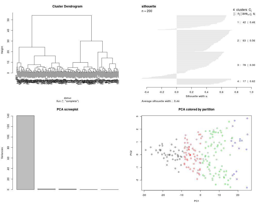
> c3 = MLearn(~CL+CW+RW, crabs, pamI(dist), k=5)
> c3
clusteringOutput: partition table

 1  2  3  4  5 
30 48 43 52 27 
The call that created this object was:
MLearn(formula = ~CL + CW + RW, data = crabs, .method = pamI(dist), 
    k = 5)
> plot(c3, data=crabs[,c("CL", "CW", "RW")])
> 
> 
> #  new interfaces to PLS thanks to Laurent Gatto
> 
> set.seed(1234)
> kp = sample(1:200, size=120)
> 
> plsda.1 = MLearn(sp~CW+RW, data=crabs, plsdaI, kp, probMethod="Bayes")
> plsda.1
MLInterfaces classification output container
The call was:
MLearn(formula = sp ~ CW + RW, data = crabs, .method = plsdaI, 
    trainInd = kp, probMethod = "Bayes")
Predicted outcome distribution for test set:

 B  O 
46 34 
Summary of scores on test set (use testScores() method for details):
        B         O 
0.4961409 0.5038591 
> confuMat(plsda.1)
     predicted
given  B  O
    B 24 13
    O 22 21
> confuMat(plsda.1,t=.65) ## requires at least 0.65 post error prob to assign species
     predicted
given  B  O NA
    B  9  4 24
    O  6 13 24
> 
> plsda.2 = MLearn(type~., data=sample.ExpressionSet[100:250,], plsdaI, 1:16)
> plsda.2
MLInterfaces classification output container
The call was:
MLearn(formula = type ~ ., data = sample.ExpressionSet[100:250, 
    ], .method = plsdaI, trainInd = 1:16)
Predicted outcome distribution for test set:

   Case Control 
      8       2 
Summary of scores on test set (use testScores() method for details):
     Case   Control 
0.8444857 0.1555143 
> confuMat(plsda.2)
         predicted
given     Case Control
  Case       4       1
  Control    4       1
> confuMat(plsda.2,t=.65) ## requires at least 0.65 post error prob to assign outcome
         predicted
given     Case Control NA
  Case       4       0  1
  Control    4       1  0
> 
> ## examples for predict
> clout <- MLearn(type~., sample.ExpressionSet[100:250,], svmI , 1:16)
> predict(clout, sample.ExpressionSet[100:250,17:26])
$testPredictions
      Q       R       S       T       U       V       W       X       Y       Z 
   Case    Case    Case    Case    Case    Case    Case Control Control    Case 
Levels: Case Control

$testScores
    Control      Case
Q 0.2031747 0.7968253
R 0.1374688 0.8625312
S 0.2118248 0.7881752
T 0.4532421 0.5467579
U 0.3712725 0.6287275
V 0.2707781 0.7292219
W 0.2680935 0.7319065
X 0.6232085 0.3767915
Y 0.5164324 0.4835676
Z 0.1082936 0.8917064

> 
> 
> 
> 
> 
> 
> dev.off()
null device 
          1 
>