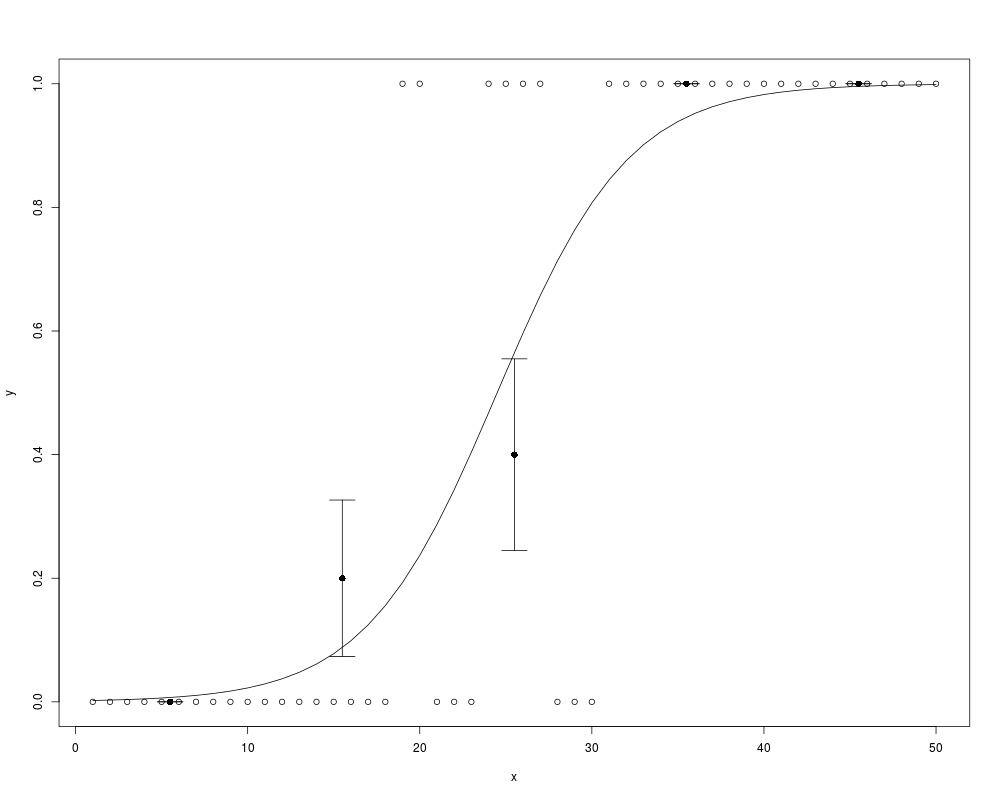
Graphical adujstment of a simple binary logistic regression to data

Description

Cuts the data into intervals, compute the response probability and its standard error for each interval and add the results to the regression curve. No test is performed but this permits to have a graphical idea of the adjustment of the model to the data.

Usage

logis.fit(model, int = 5, ...)

Arguments

Author(s)

Maxime Herv<c3><a9> <mx.herve@gmail.com>

See Also

glm

Examples

x <- 1:50
y <- c(rep(0,18),sample(0:1,14,replace=TRUE),rep(1,18))
model <- glm(y~x,family=binomial)
plot(x,y)
lines(x,model$fitted)
logis.fit(model)

Results

R version 3.3.1 (2016-06-21) -- "Bug in Your Hair"
Copyright (C) 2016 The R Foundation for Statistical Computing
Platform: x86_64-pc-linux-gnu (64-bit)

R is free software and comes with ABSOLUTELY NO WARRANTY.
You are welcome to redistribute it under certain conditions.
Type 'license()' or 'licence()' for distribution details.

R is a collaborative project with many contributors.
Type 'contributors()' for more information and
'citation()' on how to cite R or R packages in publications.

Type 'demo()' for some demos, 'help()' for on-line help, or
'help.start()' for an HTML browser interface to help.
Type 'q()' to quit R.

> library(RVAideMemoire)
*** Package RVAideMemoire v 0.9-56 ***
> png(filename="/home/ddbj/snapshot/RGM3/R_CC/result/RVAideMemoire/logis.fit.Rd_%03d_medium.png", width=480, height=480)
> ### Name: logis.fit
> ### Title: Graphical adujstment of a simple binary logistic regression to
> ###   data
> ### Aliases: logis.fit
> 
> ### ** Examples
> 
> x <- 1:50
> y <- c(rep(0,18),sample(0:1,14,replace=TRUE),rep(1,18))
> model <- glm(y~x,family=binomial)
> plot(x,y)
> lines(x,model$fitted)
> logis.fit(model)
> 
> 
> 
> 
> 
> dev.off()
null device 
          1 
>