Supported by Dr. Osamu Ogasawara and  . . |
|
Last data update: 2014.03.03 |
Random Walk on Bipartite GraphDescriptionDetects spatial outliers using Random Walk on Bipartite Graph technique Details
Author(s)Sigal Shaked & Ben Nasi Maintainer: Sigal Shaked <shaksi@post.bgu.ac.il> ReferencesLiu X., Lu C.T., Chen F.: Spatial outlier detection: Random walk based approaches. In: Proceedings of the 18th ACM SIGSPATIAL International Conference on Advances in Geographic Information Systems (ACM GIS), San Jose, CA (2010). Examples
#an example dataset:
trainSet <- cbind(
c(7.092073,7.092631,7.09263,7.093052,7.092876,7.092689,7.092515,7.092321,
7.092138,7.11455,7.11441,7.11408,7.11376,7.11338,7.11305,7.11277,7.1124,
7.11202,7.11161,7.11115,7.11068,7.11014,7.10963,7.1095,7.1089,7.10818,
7.10747,7.10674,7.116691,7.116142,7.115559,7.115007,7.114423,7.113838,
7.113272,7.112684,7.112067,7.111458,7.110869,7.110274,7.109696,7.109131,
7.109231,7.108546,7.10797,5.599215,5.597609,5.596588,5.595359,5.594478,5.593652),
c(50.77849,50.77859,50.7786,50.77878,50.77914,50.77952,50.77992,50.78035,
50.78081,53.8,53.7,53.6,53.5,54.2,55.3,55.2,56.6,57.6,57.7,58.8,59.4,59.7,
59,59.03,59.3,60.7,60.8,61.4,50.73922,50.73914,50.73905,50.73899,50.73889,
50.73881,50.73873,50.73865,50.73856,50.73847,50.73838,50.73831,50.73822,
50.73814,50.73937,50.73805,50.73798,43.2034,43.20338,43.20352,43.2037,43.20391,43.20409),
c(106.5,107.6,25,108.5,109.1,109.7,111.6,113.3,113.3,62.3,333.7,331.5,327.2,
325.5,324.8,323.5,322.3,320.3,319,317.8,316,315.1,315.3,12,312.4,311.3,310.8,
309.4,99.2,99.2,101.1,99.5,101.3,105.3,104.3,104.4,106.3,108.8,110.3,111.7,113.3,
112.1,5000,111.6,109.8,125.6,130,132.3,133.4,138,143.4),
c(0,0,1,0,0,0,0,0,0,0,0,0,0,0,0,0,0,0,0,0,0,0,0,1,0,0,0,0,0,0,0,0,0,0,0,0,0,
0,0,0,0,0,1,0,0,0,0,0,0,0,0)
)
colnames(trainSet)<- c("lng","lat","alt","isOutlier")
#first to columns of the input data are assumed to be spatial coordinates,
#and the rest are non-spatial attributes according to which outliers will be extracted
myRW <- RWBP(as.data.frame(trainSet[,1:3]), clusters.iterations=6)
#predict classification:
testPrediction<-predict(myRW,3 )
#calculate accuracy:
sum(testPrediction$class==trainSet[,"isOutlier"])/nrow(trainSet)
#confusion table
table(testPrediction$class, trainSet[,"isOutlier"])
#other options:
myRW1 <- RWBP(isOutlier~lng+lat+alt, data=as.data.frame(trainSet))
#print model summary
print(myRW1)
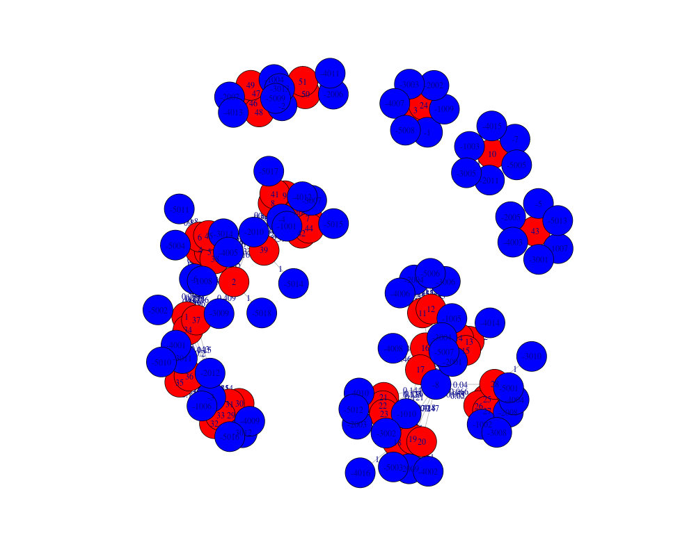
#plot model graph
plot(myRW1)
#predict probabilities of each record to be an outlier:
predict(myRW1 , top_k=4,type="prob")
Results
R version 3.3.1 (2016-06-21) -- "Bug in Your Hair"
Copyright (C) 2016 The R Foundation for Statistical Computing
Platform: x86_64-pc-linux-gnu (64-bit)

R is free software and comes with ABSOLUTELY NO WARRANTY.
You are welcome to redistribute it under certain conditions.
Type 'license()' or 'licence()' for distribution details.

R is a collaborative project with many contributors.
Type 'contributors()' for more information and
'citation()' on how to cite R or R packages in publications.

Type 'demo()' for some demos, 'help()' for on-line help, or
'help.start()' for an HTML browser interface to help.
Type 'q()' to quit R.

> library(RWBP)
Loading required package: RANN
Loading required package: igraph

Attaching package: 'igraph'

The following objects are masked from 'package:stats':

    decompose, spectrum

The following object is masked from 'package:base':

    union

Loading required package: lsa
Loading required package: SnowballC
> png(filename="/home/ddbj/snapshot/RGM3/R_CC/result/RWBP/RWBP-package.Rd_%03d_medium.png", width=480, height=480)
> ### Name: RWBP-package
> ### Title: Random Walk on Bipartite Graph
> ### Aliases: RWBP-package
> ### Keywords: spatial cluster graphs classif package
>
> ### ** Examples
>
> #an example dataset:
> trainSet <- cbind(
+ c(7.092073,7.092631,7.09263,7.093052,7.092876,7.092689,7.092515,7.092321,
+ 7.092138,7.11455,7.11441,7.11408,7.11376,7.11338,7.11305,7.11277,7.1124,
+ 7.11202,7.11161,7.11115,7.11068,7.11014,7.10963,7.1095,7.1089,7.10818,
+ 7.10747,7.10674,7.116691,7.116142,7.115559,7.115007,7.114423,7.113838,
+ 7.113272,7.112684,7.112067,7.111458,7.110869,7.110274,7.109696,7.109131,
+ 7.109231,7.108546,7.10797,5.599215,5.597609,5.596588,5.595359,5.594478,5.593652),
+ c(50.77849,50.77859,50.7786,50.77878,50.77914,50.77952,50.77992,50.78035,
+ 50.78081,53.8,53.7,53.6,53.5,54.2,55.3,55.2,56.6,57.6,57.7,58.8,59.4,59.7,
+ 59,59.03,59.3,60.7,60.8,61.4,50.73922,50.73914,50.73905,50.73899,50.73889,
+ 50.73881,50.73873,50.73865,50.73856,50.73847,50.73838,50.73831,50.73822,
+ 50.73814,50.73937,50.73805,50.73798,43.2034,43.20338,43.20352,43.2037,43.20391,43.20409),
+ c(106.5,107.6,25,108.5,109.1,109.7,111.6,113.3,113.3,62.3,333.7,331.5,327.2,
+ 325.5,324.8,323.5,322.3,320.3,319,317.8,316,315.1,315.3,12,312.4,311.3,310.8,
+ 309.4,99.2,99.2,101.1,99.5,101.3,105.3,104.3,104.4,106.3,108.8,110.3,111.7,113.3,
+ 112.1,5000,111.6,109.8,125.6,130,132.3,133.4,138,143.4),
+ c(0,0,1,0,0,0,0,0,0,0,0,0,0,0,0,0,0,0,0,0,0,0,0,1,0,0,0,0,0,0,0,0,0,0,0,0,0,
+ 0,0,0,0,0,1,0,0,0,0,0,0,0,0)
+ )
>
> colnames(trainSet)<- c("lng","lat","alt","isOutlier")
>
> #first to columns of the input data are assumed to be spatial coordinates,
> #and the rest are non-spatial attributes according to which outliers will be extracted
> myRW <- RWBP(as.data.frame(trainSet[,1:3]), clusters.iterations=6)
>
> #predict classification:
> testPrediction<-predict(myRW,3 )
> #calculate accuracy:
> sum(testPrediction$class==trainSet[,"isOutlier"])/nrow(trainSet)
[1] 0.9215686
> #confusion table
> table(testPrediction$class, trainSet[,"isOutlier"])

     0  1
  0 46  2
  1  2  1
>
> #other options:
> myRW1 <- RWBP(isOutlier~lng+lat+alt, data=as.data.frame(trainSet))
> #print model summary
> print(myRW1)
 A Random Walk on Bipartite Graph spatial outlier detection model was built:
 ----------------------------------------------------------------------------

 neighberhood size =  10
 initial clusters amount =  8
 each process increases clusters amount by  2  more clusters
 clusters iterations amount =  6
 alfa =  0.5
 dumping factor =  0.9
 valid rows =  51  out of  51  input rows (records with empty values were removed)

 a bipartite graph was built:
IGRAPH UNWB 129 306 --
+ attr: name (v/c), type (v/l), RW.Y (e/n), avgDist (e/n), weight (e/n)
+ edges (vertex names):
 [1] 1 ---4    2 ---5    3 ---8    4 ---5    5 ---5    6 ---5    7 ---5
 [8] 8 ---5    9 ---5    10---8    11---7    12---7    13---7    14---7
[15] 15---7    16---7    17---6    18---6    19---6    20---6    21---6
[22] 22---6    23---6    24---8    25---1    26---1    27---1    28---1
[29] 29---4    30---4    31---4    32---4    33---4    34---4    35---4
[36] 36---4    37---4    38---5    39---5    40---5    41---5    42---5
[43] 43---3    44---5    45---5    46---2    47---2    48---2    49---2
[50] 50---2    51---2    1 ---1003 2 ---1001 3 ---1010 4 ---1001 5 ---1001
+ ... omitted several edges

 outlier scores:
      row_num outlierScore
 [1,]      43    0.5971466
 [2,]      10    0.6038678
 [3,]      46    0.7125017
 [4,]      11    0.7527546
 [5,]      12    0.7528352
 [6,]       3    0.7536465
 [7,]      28    0.7871346
 [8,]      24    0.7875049
 [9,]      15    0.9116267
[10,]      13    0.9126523
[11,]      14    0.9131557
[12,]      16    0.9138868
[13,]       4    0.9254196
[14,]       1    0.9264440
[15,]       6    0.9264844
[16,]       8    0.9269722
[17,]       9    0.9269722
[18,]       7    0.9270987
[19,]       2    0.9272290
[20,]       5    0.9273845
[21,]      45    0.9472854
[22,]      37    0.9479707
[23,]      39    0.9482102
[24,]      38    0.9482658
[25,]      41    0.9482847
[26,]      42    0.9485131
[27,]      40    0.9485152
[28,]      44    0.9486894
[29,]      27    0.9531621
[30,]      26    0.9535070
[31,]      21    0.9549538
[32,]      25    0.9559935
[33,]      22    0.9561667
[34,]      51    0.9565273
[35,]      50    0.9565957
[36,]      47    0.9589698
[37,]      48    0.9595243
[38,]      49    0.9606545
[39,]      18    0.9750983
[40,]      20    0.9754692
[41,]      23    0.9769280
[42,]      19    0.9772926
[43,]      17    0.9773157
[44,]      33    0.9960896
[45,]      31    0.9963835
[46,]      34    0.9970310
[47,]      36    0.9977316
[48,]      29    0.9978277
[49,]      30    0.9978277
[50,]      32    0.9978818
[51,]      35    0.9979112
> #plot model graph
> plot(myRW1)
> #predict probabilities of each record to be an outlier:
> predict(myRW1 , top_k=4,type="prob")
        lng      lat    alt         prob
1  7.092073 50.77849  106.5 0.1783270104
2  7.092631 50.77859  107.6 0.1763683100
3  7.092630 50.77860   25.0 0.6094966656
4  7.093052 50.77878  108.5 0.1808832377
5  7.092876 50.77914  109.1 0.1759803769
6  7.092689 50.77952  109.7 0.1782261956
7  7.092515 50.77992  111.6 0.1766933551
8  7.092321 50.78035  113.3 0.1770090751
9  7.092138 50.78081  113.3 0.1770090751
10 7.114550 53.80000   62.3 0.9832289511
11 7.114410 53.70000  333.7 0.6117221906
12 7.114080 53.60000  331.5 0.6115210887
13 7.113760 53.50000  327.2 0.2127404244
14 7.113380 54.20000  325.5 0.2114844184
15 7.113050 55.30000  324.8 0.2152997005
16 7.112770 55.20000  323.5 0.2096602602
17 7.112400 56.60000  322.3 0.0513904909
18 7.112020 57.60000  320.3 0.0569234385
19 7.111610 57.70000  319.0 0.0514480669
20 7.111150 58.80000  317.8 0.0559977735
21 7.110680 59.40000  316.0 0.1071885364
22 7.110140 59.70000  315.1 0.1041619371
23 7.109630 59.00000  315.3 0.0523577516
24 7.109500 59.03000   12.0 0.5250120865
25 7.108900 59.30000  312.4 0.1045942806
26 7.108180 60.70000  311.3 0.1107986809
27 7.107470 60.80000  310.8 0.1116591940
28 7.106740 61.40000  309.4 0.5259361223
29 7.116691 50.73922   99.2 0.0002083576
30 7.116142 50.73914   99.2 0.0002083576
31 7.115559 50.73905  101.1 0.0038119814
32 7.115007 50.73899   99.5 0.0000731755
33 7.114423 50.73889  101.3 0.0045453478
34 7.113838 50.73881  105.3 0.0021963197
35 7.113272 50.73873  104.3 0.0000000000
36 7.112684 50.73865  104.4 0.0004480287
37 7.112067 50.73856  106.3 0.1246129658
38 7.111458 50.73847  108.8 0.1238766162
39 7.110869 50.73838  110.3 0.1240152856
40 7.110274 50.73831  111.7 0.1232544232
41 7.109696 50.73822  113.3 0.1238293756
42 7.109131 50.73814  112.1 0.1232596502
43 7.109231 50.73937 5000.0 1.0000000000
44 7.108546 50.73805  111.6 0.1228196936
45 7.107970 50.73798  109.8 0.1263230607
46 5.599215 43.20340  125.6 0.7121623470
47 5.597609 43.20338  130.0 0.0971676378
48 5.596588 43.20352  132.3 0.0957841237
49 5.595359 43.20370  133.4 0.0929638987
50 5.594478 43.20391  138.0 0.1030916573
51 5.593652 43.20409  143.4 0.1032622912
>
>
>
>
>
> dev.off()
null device
          1
>
|
Created & Maintained by Osamu Ogasawara (osamu.ogasawara@gmail.com) and 