R Graphical Manual

Browse All

Last data update: 2014.03.03

R: Random Walk on Bipartite Graph

RWBP	R Documentation

Random Walk on Bipartite Graph

Description

Performs an outlier detection on a given data frame/matrix.

Usage

RWBP(x,...,nn_k,min.clusters,clusters.iterations,
clusters.stepSize,alfa,dumping.factor)
## Default S3 method:
RWBP(x,...,nn_k=10,min.clusters=8,clusters.iterations=6,
clusters.stepSize=2,alfa=0.5,dumping.factor=0.9)
## S3 method for class 'formula'
RWBP(formula,data,...,nn_k=10,min.clusters=8,clusters.iterations=6,
clusters.stepSize=2,alfa=0.5,dumping.factor=0.9)
## S3 method for class 'RWBP'
print(x, ...)
## S3 method for class 'RWBP'
plot(x, ...)

Arguments

`formula`	a formula representation of the problem (the dependent variable (y) will be ignored, the first two x attributes have to be spatial coordinates and the rest are numeric attributes)
`data`	a data frame containing the data to be analysed (may contain additional columns).
`x`	a data frame containing the data to be analysed. the first two columns must be spatial coordinates and the other columns are non-spatial attributes on which we search for outliers
`nn_k`	neighbourhood size (for finding each objects k nearest neighbours)
`min.clusters`	the number of clusters in the first clustering process
`clusters.iterations`	the number of clustering process to be conducted
`clusters.stepSize`	increase the amount of clusters in the following clustering process by this size
`alfa`	helps to compute more accurate edge value (distance between object and cluster)
`dumping.factor`	dumping factor (the probability to return to the original node during each step along a random walk)
`...`	currently not in use

Details

A spatial outlier detection approach based on RW techniques. A Bipartite graph is constructed based on the spatial and/or non-spatial attributes of the spatial objects in the dataset. Secondly, RW techniques are utilized on the graphs to compute the outlierness for each point (the differences between spatial objects and their spatial neighbours). The top k objects with higher outlierness are recognized as outliers.

Value

Returns as RWBP object that contains several components:

`data`	the data after removing records with empty fields
`X`	a data frame containing the spatial attributes(first two columns) from the input data
`Y`	a data frame containing the non-spatial attributes(all but the first two columns) from the input data
`ID`	a vector with sequential numbers, used as an index
`n`	number of valid records
`n.orig`	number of records accepted in the input data
`nn_k`	neighbourhood size for knn search
`k`	clusters amount in the first clustering process
`clusters.stepSize`	each next clustering process is increased by this size
`h`	number of conducted clustering processes
`alfa`	Helps to compute more accurate edge value (distance between object and cluster)
`c`	Dumping factor (the probability to return to the original node during each step along a random walk)
`nearest.indexes`	a matrix where each row contains a spatial object's nn_k nearest neighbours
`clusteredData`	a data frame containing the results of all clustering process: an object, the cluster it belongs to and the distance between the two
`igraph`	an igraph object built according to the connections between spatial objects and clusters
`OutScore`	the outlierness scores of each record, sorted ascending by score, the first column is the index of the record and the second column is the given score
`objects.similarity`	a matrix where each row holds the similarity between a spatial object and its nn_k neighbours

Note

First two columns must be spatial coordinates, and the rest of the columns must be numeric attributes. records with empty fields are removed from the input data.

Author(s)

Sigal Shaked & Ben Nasi

References

Liu X., Lu C.T., Chen F.: Spatial outlier detection: Random walk based approaches. In: Proceedings of the 18th ACM SIGSPATIAL International Conference on Advances in Geographic Information Systems (ACM GIS), San Jose, CA (2010).

Examples

#an example dataset:
trainSet <- cbind(
c(7.092073,7.092631,7.09263,7.093052,7.092876,7.092689,7.092515,7.092321,
7.092138,7.11455,7.11441,7.11408,7.11376,7.11338,7.11305,7.11277,7.1124,
7.11202,7.11161,7.11115,7.11068,7.11014,7.10963,7.1095,7.1089,7.10818,
7.10747,7.10674,7.116691,7.116142,7.115559,7.115007,7.114423,7.113838,
7.113272,7.112684,7.112067,7.111458,7.110869,7.110274,7.109696,7.109131,
7.109231,7.108546,7.10797,5.599215,5.597609,5.596588,5.595359,5.594478,5.593652),
c(50.77849,50.77859,50.7786,50.77878,50.77914,50.77952,50.77992,50.78035,
50.78081,53.8,53.7,53.6,53.5,54.2,55.3,55.2,56.6,57.6,57.7,58.8,59.4,59.7,
59,59.03,59.3,60.7,60.8,61.4,50.73922,50.73914,50.73905,50.73899,50.73889,
50.73881,50.73873,50.73865,50.73856,50.73847,50.73838,50.73831,50.73822,
50.73814,50.73937,50.73805,50.73798,43.2034,43.20338,43.20352,43.2037,43.20391,43.20409),
c(106.5,107.6,25,108.5,109.1,109.7,111.6,113.3,113.3,62.3,333.7,331.5,327.2,
325.5,324.8,323.5,322.3,320.3,319,317.8,316,315.1,315.3,12,312.4,311.3,310.8,
309.4,99.2,99.2,101.1,99.5,101.3,105.3,104.3,104.4,106.3,108.8,110.3,111.7,113.3,
112.1,5000,111.6,109.8,125.6,130,132.3,133.4,138,143.4),
c(0,0,1,0,0,0,0,0,0,0,0,0,0,0,0,0,0,0,0,0,0,0,0,1,0,0,0,0,0,0,0,0,0,0,0,0,0,
0,0,0,0,0,1,0,0,0,0,0,0,0,0)
)

colnames(trainSet)<- c("lng","lat","alt","isOutlier")

#first to columns of the input data are assumed to be spatial coordinates, 
#and the rest are non-spatial attributes according to which outliers will be extracted
myRW <- RWBP(as.data.frame(trainSet[,1:3]), clusters.iterations=6)

#predict classification:
testPrediction<-predict(myRW,3 )
#calculate accuracy:
sum(testPrediction$class==trainSet[,"isOutlier"])/nrow(trainSet)
#confusion table
table(testPrediction$class, trainSet[,"isOutlier"])

#other options:
myRW1 <- RWBP(isOutlier~lng+lat+alt, data=as.data.frame(trainSet))
#print model summary
print(myRW1)
#plot model graph
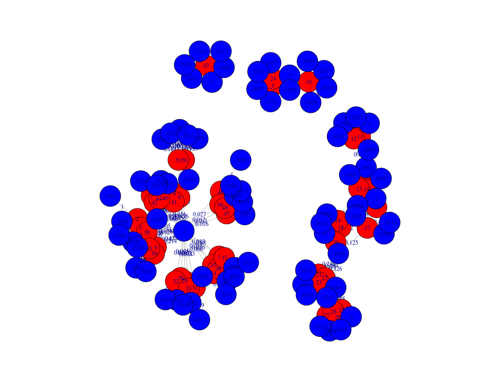
plot(myRW1)
#predict probabilities of each record to be an outlier:
predict(myRW1 , top_k=4,type="prob")

Results


R version 3.3.1 (2016-06-21) -- "Bug in Your Hair"
Copyright (C) 2016 The R Foundation for Statistical Computing
Platform: x86_64-pc-linux-gnu (64-bit)

R is free software and comes with ABSOLUTELY NO WARRANTY.
You are welcome to redistribute it under certain conditions.
Type 'license()' or 'licence()' for distribution details.

R is a collaborative project with many contributors.
Type 'contributors()' for more information and
'citation()' on how to cite R or R packages in publications.

Type 'demo()' for some demos, 'help()' for on-line help, or
'help.start()' for an HTML browser interface to help.
Type 'q()' to quit R.

> library(RWBP)
Loading required package: RANN
Loading required package: igraph

Attaching package: 'igraph'

The following objects are masked from 'package:stats':

    decompose, spectrum

The following object is masked from 'package:base':

    union

Loading required package: lsa
Loading required package: SnowballC
> png(filename="/home/ddbj/snapshot/RGM3/R_CC/result/RWBP/RWBP.Rd_%03d_medium.png", width=480, height=480)
> ### Name: RWBP
> ### Title: Random Walk on Bipartite Graph
> ### Aliases: RWBP RWBP.default RWBP.formula print.RWBP plot.RWBP
> ### Keywords: spatial cluster graphs classif
> 
> ### ** Examples
> 
> #an example dataset:
> trainSet <- cbind(
+ c(7.092073,7.092631,7.09263,7.093052,7.092876,7.092689,7.092515,7.092321,
+ 7.092138,7.11455,7.11441,7.11408,7.11376,7.11338,7.11305,7.11277,7.1124,
+ 7.11202,7.11161,7.11115,7.11068,7.11014,7.10963,7.1095,7.1089,7.10818,
+ 7.10747,7.10674,7.116691,7.116142,7.115559,7.115007,7.114423,7.113838,
+ 7.113272,7.112684,7.112067,7.111458,7.110869,7.110274,7.109696,7.109131,
+ 7.109231,7.108546,7.10797,5.599215,5.597609,5.596588,5.595359,5.594478,5.593652),
+ c(50.77849,50.77859,50.7786,50.77878,50.77914,50.77952,50.77992,50.78035,
+ 50.78081,53.8,53.7,53.6,53.5,54.2,55.3,55.2,56.6,57.6,57.7,58.8,59.4,59.7,
+ 59,59.03,59.3,60.7,60.8,61.4,50.73922,50.73914,50.73905,50.73899,50.73889,
+ 50.73881,50.73873,50.73865,50.73856,50.73847,50.73838,50.73831,50.73822,
+ 50.73814,50.73937,50.73805,50.73798,43.2034,43.20338,43.20352,43.2037,43.20391,43.20409),
+ c(106.5,107.6,25,108.5,109.1,109.7,111.6,113.3,113.3,62.3,333.7,331.5,327.2,
+ 325.5,324.8,323.5,322.3,320.3,319,317.8,316,315.1,315.3,12,312.4,311.3,310.8,
+ 309.4,99.2,99.2,101.1,99.5,101.3,105.3,104.3,104.4,106.3,108.8,110.3,111.7,113.3,
+ 112.1,5000,111.6,109.8,125.6,130,132.3,133.4,138,143.4),
+ c(0,0,1,0,0,0,0,0,0,0,0,0,0,0,0,0,0,0,0,0,0,0,0,1,0,0,0,0,0,0,0,0,0,0,0,0,0,
+ 0,0,0,0,0,1,0,0,0,0,0,0,0,0)
+ )
> 
> colnames(trainSet)<- c("lng","lat","alt","isOutlier")
> 
> #first to columns of the input data are assumed to be spatial coordinates, 
> #and the rest are non-spatial attributes according to which outliers will be extracted
> myRW <- RWBP(as.data.frame(trainSet[,1:3]), clusters.iterations=6)
> 
> #predict classification:
> testPrediction<-predict(myRW,3 )
> #calculate accuracy:
> sum(testPrediction$class==trainSet[,"isOutlier"])/nrow(trainSet)
[1] 0.9215686
> #confusion table
> table(testPrediction$class, trainSet[,"isOutlier"])
   
     0  1
  0 46  2
  1  2  1
> 
> #other options:
> myRW1 <- RWBP(isOutlier~lng+lat+alt, data=as.data.frame(trainSet))
> #print model summary
> print(myRW1)
 A Random Walk on Bipartite Graph spatial outlier detection model was built: 
 ---------------------------------------------------------------------------- 

 neighberhood size =  10 
 initial clusters amount =  8 
 each process increases clusters amount by  2  more clusters
 clusters iterations amount =  6 
 alfa =  0.5 
 dumping factor =  0.9 
 valid rows =  51  out of  51  input rows (records with empty values were removed) 

 a bipartite graph was built: 
IGRAPH UNWB 129 306 -- 
+ attr: name (v/c), type (v/l), RW.Y (e/n), avgDist (e/n), weight (e/n)
+ edges (vertex names):
 [1] 1 ---7    2 ---4    3 ---6    4 ---4    5 ---4    6 ---4    7 ---4   
 [8] 8 ---4    9 ---4    10---6    11---1    12---1    13---1    14---1   
[15] 15---1    16---1    17---1    18---5    19---5    20---5    21---5   
[22] 22---5    23---5    24---6    25---5    26---5    27---5    28---5   
[29] 29---7    30---7    31---7    32---7    33---7    34---7    35---7   
[36] 36---7    37---7    38---4    39---4    40---4    41---4    42---4   
[43] 43---3    44---4    45---4    46---8    47---8    48---8    49---8   
[50] 50---2    51---2    1 ---1004 2 ---1004 3 ---1010 4 ---1004 5 ---1004
+ ... omitted several edges

 outlier scores:  
      row_num outlierScore
 [1,]      43    0.5833527
 [2,]      10    0.6089308
 [3,]      28    0.7131929
 [4,]      39    0.7636134
 [5,]      46    0.8019707
 [6,]       3    0.9166680
 [7,]      45    0.9265279
 [8,]      41    0.9274554
 [9,]      38    0.9275253
[10,]      40    0.9280429
[11,]      44    0.9283606
[12,]      42    0.9284286
[13,]      37    0.9284734
[14,]      11    0.9417769
[15,]      12    0.9418158
[16,]       4    0.9422665
[17,]       6    0.9437767
[18,]       8    0.9442862
[19,]       9    0.9442862
[20,]       7    0.9446939
[21,]       5    0.9448643
[22,]       1    0.9450141
[23,]       2    0.9451091
[24,]      15    0.9459708
[25,]      16    0.9463177
[26,]      14    0.9471142
[27,]      13    0.9472698
[28,]      24    0.9531562
[29,]      26    0.9610300
[30,]      27    0.9622911
[31,]      22    0.9629771
[32,]      21    0.9634017
[33,]      25    0.9636330
[34,]      51    0.9698829
[35,]      50    0.9699811
[36,]      47    0.9707877
[37,]      49    0.9713708
[38,]      48    0.9729328
[39,]      34    0.9750084
[40,]      31    0.9753471
[41,]      33    0.9753855
[42,]      32    0.9765985
[43,]      29    0.9766186
[44,]      30    0.9766186
[45,]      36    0.9770936
[46,]      35    0.9771440
[47,]      19    0.9902121
[48,]      17    0.9944830
[49,]      23    0.9947393
[50,]      20    0.9958984
[51,]      18    0.9964122
> #plot model graph
> plot(myRW1)
> #predict probabilities of each record to be an outlier:
> predict(myRW1 , top_k=4,type="prob")
        lng      lat    alt        prob
1  7.092073 50.77849  106.5 0.124432665
2  7.092631 50.77859  107.6 0.124202688
3  7.092630 50.77860   25.0 0.193057510
4  7.093052 50.77878  108.5 0.131084593
5  7.092876 50.77914  109.1 0.124795352
6  7.092689 50.77952  109.7 0.127428371
7  7.092515 50.77992  111.6 0.125207940
8  7.092321 50.78035  113.3 0.126194987
9  7.092138 50.78081  113.3 0.126194987
10 7.114550 53.80000   62.3 0.938076611
11 7.114410 53.70000  333.7 0.132269917
12 7.114080 53.60000  331.5 0.132175755
13 7.113760 53.50000  327.2 0.118971843
14 7.113380 54.20000  325.5 0.119348394
15 7.113050 55.30000  324.8 0.122116590
16 7.112770 55.20000  323.5 0.121276823
17 7.112400 56.60000  322.3 0.004670599
18 7.112020 57.60000  320.3 0.000000000
19 7.111610 57.70000  319.0 0.015010350
20 7.111150 58.80000  317.8 0.001243936
21 7.110680 59.40000  316.0 0.079917039
22 7.110140 59.70000  315.1 0.080945041
23 7.109630 59.00000  315.3 0.004050160
24 7.109500 59.03000   12.0 0.104721019
25 7.108900 59.30000  312.4 0.079357268
26 7.108180 60.70000  311.3 0.085658815
27 7.107470 60.80000  310.8 0.082605732
28 7.106740 61.40000  309.4 0.685662351
29 7.116691 50.73922   99.2 0.047919467
30 7.116142 50.73914   99.2 0.047919467
31 7.115559 50.73905  101.1 0.050997736
32 7.115007 50.73899   99.5 0.047968336
33 7.114423 50.73889  101.3 0.050904945
34 7.113838 50.73881  105.3 0.051817812
35 7.113272 50.73873  104.3 0.046647638
36 7.112684 50.73865  104.4 0.046769712
37 7.112067 50.73856  106.3 0.164477111
38 7.111458 50.73847  108.8 0.166772344
39 7.110869 50.73838  110.3 0.563596375
40 7.110274 50.73831  111.7 0.165519381
41 7.109696 50.73822  113.3 0.166941715
42 7.109131 50.73814  112.1 0.164585456
43 7.109231 50.73937 5000.0 1.000000000
44 7.108546 50.73805  111.6 0.164750077
45 7.107970 50.73798  109.8 0.169186987
46 5.599215 43.20340  125.6 0.470734947
47 5.597609 43.20338  130.0 0.062036041
48 5.596588 43.20352  132.3 0.056842636
49 5.595359 43.20370  133.4 0.060624216
50 5.594478 43.20391  138.0 0.063988574
51 5.593652 43.20409  143.4 0.064226490
> 
> 
> 
> 
> 
> dev.off()
null device 
          1 
>