predict.RWBP

Description

Predict spatial outliers according to a RWBP model

Usage

## S3 method for class 'RWBP'
predict(object, top_k = 3, type = "raw", ...)

Arguments

Value

Returns the input data frame/matrix with an additional column that contains the prediction results. The additional column is set according to the type parameter:

Author(s)

Sigal Shaked & Ben Nasi

References

Liu X., Lu C.T., Chen F.: Spatial outlier detection: Random walk based approaches. In: Proceedings of the 18th ACM SIGSPATIAL International Conference on Advances in Geographic Information Systems (ACM GIS), San Jose, CA (2010).

See Also

RWBP,RWBP-package

Examples

#an example dataset:
trainSet <- cbind(
c(7.092073,7.092631,7.09263,7.093052,7.092876,7.092689,7.092515,7.092321,
7.092138,7.11455,7.11441,7.11408,7.11376,7.11338,7.11305,7.11277,7.1124,
7.11202,7.11161,7.11115,7.11068,7.11014,7.10963,7.1095,7.1089,7.10818,
7.10747,7.10674,7.116691,7.116142,7.115559,7.115007,7.114423,7.113838,
7.113272,7.112684,7.112067,7.111458,7.110869,7.110274,7.109696,7.109131,
7.109231,7.108546,7.10797,5.599215,5.597609,5.596588,5.595359,5.594478,5.593652),
c(50.77849,50.77859,50.7786,50.77878,50.77914,50.77952,50.77992,50.78035,
50.78081,53.8,53.7,53.6,53.5,54.2,55.3,55.2,56.6,57.6,57.7,58.8,59.4,59.7,
59,59.03,59.3,60.7,60.8,61.4,50.73922,50.73914,50.73905,50.73899,50.73889,
50.73881,50.73873,50.73865,50.73856,50.73847,50.73838,50.73831,50.73822,
50.73814,50.73937,50.73805,50.73798,43.2034,43.20338,43.20352,43.2037,43.20391,43.20409),
c(106.5,107.6,25,108.5,109.1,109.7,111.6,113.3,113.3,62.3,333.7,331.5,327.2,
325.5,324.8,323.5,322.3,320.3,319,317.8,316,315.1,315.3,12,312.4,311.3,310.8,
309.4,99.2,99.2,101.1,99.5,101.3,105.3,104.3,104.4,106.3,108.8,110.3,111.7,113.3,
112.1,5000,111.6,109.8,125.6,130,132.3,133.4,138,143.4),
c(0,0,1,0,0,0,0,0,0,0,0,0,0,0,0,0,0,0,0,0,0,0,0,1,0,0,0,0,0,0,0,0,0,0,0,0,0,
0,0,0,0,0,1,0,0,0,0,0,0,0,0)
)

colnames(trainSet)<- c("lng","lat","alt","isOutlier")

#first to columns of the input data are assumed to be spatial coordinates, 
#and the rest are non-spatial attributes according to which outliers will be extracted
myRW <- RWBP(as.data.frame(trainSet[,1:3]), clusters.iterations=6)

#predict classification:
testPrediction<-predict(myRW,3 )
#calculate accuracy:
sum(testPrediction$class==trainSet[,"isOutlier"])/nrow(trainSet)
#confusion table
table(testPrediction$class, trainSet[,"isOutlier"])

#other options:
myRW1 <- RWBP(isOutlier~lng+lat+alt, data=as.data.frame(trainSet))
#print model summary
print(myRW1)
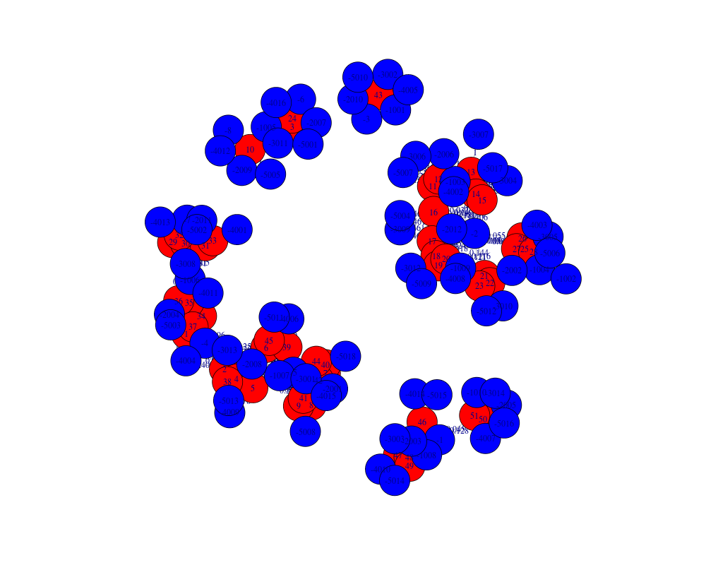
#plot model graph
plot(myRW1)
#predict probabilities of each record to be an outlier:
predict(myRW1 , top_k=4,type="prob")

Results

R version 3.3.1 (2016-06-21) -- "Bug in Your Hair"
Copyright (C) 2016 The R Foundation for Statistical Computing
Platform: x86_64-pc-linux-gnu (64-bit)

R is free software and comes with ABSOLUTELY NO WARRANTY.
You are welcome to redistribute it under certain conditions.
Type 'license()' or 'licence()' for distribution details.

R is a collaborative project with many contributors.
Type 'contributors()' for more information and
'citation()' on how to cite R or R packages in publications.

Type 'demo()' for some demos, 'help()' for on-line help, or
'help.start()' for an HTML browser interface to help.
Type 'q()' to quit R.

> library(RWBP)
Loading required package: RANN
Loading required package: igraph

Attaching package: 'igraph'

The following objects are masked from 'package:stats':

    decompose, spectrum

The following object is masked from 'package:base':

    union

Loading required package: lsa
Loading required package: SnowballC
> png(filename="/home/ddbj/snapshot/RGM3/R_CC/result/RWBP/predict.RWBP.Rd_%03d_medium.png", width=480, height=480)
> ### Name: predict.RWBP
> ### Title: predict.RWBP
> ### Aliases: predict.RWBP
> ### Keywords: spatial cluster graphs classif
> 
> ### ** Examples
> 
> #an example dataset:
> trainSet <- cbind(
+ c(7.092073,7.092631,7.09263,7.093052,7.092876,7.092689,7.092515,7.092321,
+ 7.092138,7.11455,7.11441,7.11408,7.11376,7.11338,7.11305,7.11277,7.1124,
+ 7.11202,7.11161,7.11115,7.11068,7.11014,7.10963,7.1095,7.1089,7.10818,
+ 7.10747,7.10674,7.116691,7.116142,7.115559,7.115007,7.114423,7.113838,
+ 7.113272,7.112684,7.112067,7.111458,7.110869,7.110274,7.109696,7.109131,
+ 7.109231,7.108546,7.10797,5.599215,5.597609,5.596588,5.595359,5.594478,5.593652),
+ c(50.77849,50.77859,50.7786,50.77878,50.77914,50.77952,50.77992,50.78035,
+ 50.78081,53.8,53.7,53.6,53.5,54.2,55.3,55.2,56.6,57.6,57.7,58.8,59.4,59.7,
+ 59,59.03,59.3,60.7,60.8,61.4,50.73922,50.73914,50.73905,50.73899,50.73889,
+ 50.73881,50.73873,50.73865,50.73856,50.73847,50.73838,50.73831,50.73822,
+ 50.73814,50.73937,50.73805,50.73798,43.2034,43.20338,43.20352,43.2037,43.20391,43.20409),
+ c(106.5,107.6,25,108.5,109.1,109.7,111.6,113.3,113.3,62.3,333.7,331.5,327.2,
+ 325.5,324.8,323.5,322.3,320.3,319,317.8,316,315.1,315.3,12,312.4,311.3,310.8,
+ 309.4,99.2,99.2,101.1,99.5,101.3,105.3,104.3,104.4,106.3,108.8,110.3,111.7,113.3,
+ 112.1,5000,111.6,109.8,125.6,130,132.3,133.4,138,143.4),
+ c(0,0,1,0,0,0,0,0,0,0,0,0,0,0,0,0,0,0,0,0,0,0,0,1,0,0,0,0,0,0,0,0,0,0,0,0,0,
+ 0,0,0,0,0,1,0,0,0,0,0,0,0,0)
+ )
> 
> colnames(trainSet)<- c("lng","lat","alt","isOutlier")
> 
> #first to columns of the input data are assumed to be spatial coordinates, 
> #and the rest are non-spatial attributes according to which outliers will be extracted
> myRW <- RWBP(as.data.frame(trainSet[,1:3]), clusters.iterations=6)
> 
> #predict classification:
> testPrediction<-predict(myRW,3 )
> #calculate accuracy:
> sum(testPrediction$class==trainSet[,"isOutlier"])/nrow(trainSet)
[1] 0.9215686
> #confusion table
> table(testPrediction$class, trainSet[,"isOutlier"])
   
     0  1
  0 46  2
  1  2  1
> 
> #other options:
> myRW1 <- RWBP(isOutlier~lng+lat+alt, data=as.data.frame(trainSet))
> #print model summary
> print(myRW1)
 A Random Walk on Bipartite Graph spatial outlier detection model was built: 
 ---------------------------------------------------------------------------- 

 neighberhood size =  10 
 initial clusters amount =  8 
 each process increases clusters amount by  2  more clusters
 clusters iterations amount =  6 
 alfa =  0.5 
 dumping factor =  0.9 
 valid rows =  51  out of  51  input rows (records with empty values were removed) 

 a bipartite graph was built: 
IGRAPH UNWB 129 306 -- 
+ attr: name (v/c), type (v/l), RW.Y (e/n), avgDist (e/n), weight (e/n)
+ edges (vertex names):
 [1] 1 ---3    2 ---3    3 ---4    4 ---3    5 ---3    6 ---3    7 ---6   
 [8] 8 ---6    9 ---6    10---4    11---1    12---1    13---1    14---1   
[15] 15---1    16---1    17---1    18---1    19---1    20---1    21---1   
[22] 22---1    23---1    24---4    25---1    26---1    27---1    28---1   
[29] 29---5    30---5    31---5    32---5    33---5    34---3    35---5   
[36] 36---5    37---3    38---3    39---6    40---6    41---6    42---6   
[43] 43---2    44---6    45---3    46---8    47---8    48---8    49---8   
[50] 50---7    51---7    1 ---1005 2 ---1010 3 ---1006 4 ---1010 5 ---1010
+ ... omitted several edges

 outlier scores:  
      row_num outlierScore
 [1,]      43    0.5828438
 [2,]      10    0.5959659
 [3,]      46    0.6677292
 [4,]      51    0.7448139
 [5,]      50    0.7451195
 [6,]      42    0.7635689
 [7,]      13    0.7637470
 [8,]      28    0.8026196
 [9,]      47    0.9004970
[10,]      48    0.9009951
[11,]      49    0.9020957
[12,]       3    0.9167528
[13,]      11    0.9241027
[14,]      12    0.9242176
[15,]      38    0.9258850
[16,]      45    0.9267420
[17,]      15    0.9268838
[18,]      41    0.9270466
[19,]      40    0.9274883
[20,]      37    0.9275324
[21,]      44    0.9275440
[22,]      39    0.9277220
[23,]      16    0.9285311
[24,]      14    0.9289535
[25,]       4    0.9440723
[26,]       1    0.9441995
[27,]       7    0.9442752
[28,]       8    0.9442924
[29,]       9    0.9442924
[30,]       5    0.9444460
[31,]       6    0.9444807
[32,]       2    0.9452129
[33,]      24    0.9652561
[34,]      26    0.9744550
[35,]      27    0.9751114
[36,]      22    0.9754449
[37,]      21    0.9756838
[38,]      25    0.9757264
[39,]      20    0.9950154
[40,]      18    0.9950273
[41,]      19    0.9950798
[42,]      17    0.9951369
[43,]      34    0.9960694
[44,]      23    0.9962027
[45,]      36    0.9976380
[46,]      32    0.9978886
[47,]      35    0.9979231
[48,]      33    0.9979525
[49,]      31    0.9982022
[50,]      29    0.9982347
[51,]      30    0.9982347
> #plot model graph
> plot(myRW1)
> #predict probabilities of each record to be an outlier:
> predict(myRW1 , top_k=4,type="prob")
        lng      lat    alt         prob
1  7.092073 50.77849  106.5 1.300827e-01
2  7.092631 50.77859  107.6 1.276431e-01
3  7.092630 50.77860   25.0 1.961572e-01
4  7.093052 50.77878  108.5 1.303889e-01
5  7.092876 50.77914  109.1 1.294892e-01
6  7.092689 50.77952  109.7 1.294059e-01
7  7.092515 50.77992  111.6 1.299005e-01
8  7.092321 50.78035  113.3 1.298591e-01
9  7.092138 50.78081  113.3 1.298591e-01
10 7.114550 53.80000   62.3 9.684104e-01
11 7.114410 53.70000  333.7 1.784632e-01
12 7.114080 53.60000  331.5 1.781865e-01
13 7.113760 53.50000  327.2 5.644990e-01
14 7.113380 54.20000  325.5 1.667856e-01
15 7.113050 55.30000  324.8 1.717681e-01
16 7.112770 55.20000  323.5 1.678024e-01
17 7.112400 56.60000  322.3 7.457538e-03
18 7.112020 57.60000  320.3 7.721361e-03
19 7.111610 57.70000  319.0 7.594868e-03
20 7.111150 58.80000  317.8 7.749967e-03
21 7.110680 59.40000  316.0 5.428830e-02
22 7.110140 59.70000  315.1 5.486357e-02
23 7.109630 59.00000  315.3 4.891774e-03
24 7.109500 59.03000   12.0 7.939170e-02
25 7.108900 59.30000  312.4 5.418585e-02
26 7.108180 60.70000  311.3 5.724653e-02
27 7.107470 60.80000  310.8 5.566640e-02
28 7.106740 61.40000  309.4 4.709182e-01
29 7.116691 50.73922   99.2 0.000000e+00
30 7.116142 50.73914   99.2 0.000000e+00
31 7.115559 50.73905  101.1 7.811665e-05
32 7.115007 50.73899   99.5 8.332474e-04
33 7.114423 50.73889  101.3 6.792594e-04
34 7.113838 50.73881  105.3 5.212603e-03
35 7.113272 50.73873  104.3 7.499900e-04
36 7.112684 50.73865  104.4 1.436439e-03
37 7.112067 50.73856  106.3 1.702065e-01
38 7.111458 50.73847  108.8 1.741726e-01
39 7.110869 50.73838  110.3 1.697503e-01
40 7.110274 50.73831  111.7 1.703129e-01
41 7.109696 50.73822  113.3 1.713762e-01
42 7.109131 50.73814  112.1 5.649276e-01
43 7.109231 50.73937 5000.0 1.000000e+00
44 7.108546 50.73805  111.6 1.701787e-01
45 7.107970 50.73798  109.8 1.721094e-01
46 5.599215 43.20340  125.6 7.956493e-01
47 5.597609 43.20338  130.0 2.352909e-01
48 5.596588 43.20352  132.3 2.340919e-01
49 5.595359 43.20370  133.4 2.314422e-01
50 5.594478 43.20391  138.0 6.093423e-01
51 5.593652 43.20409  143.4 6.100780e-01
> 
> 
> 
> 
> 
> dev.off()
null device 
          1 
>