Supported by Dr. Osamu Ogasawara and  . . |
|
Last data update: 2014.03.03 |
R/Weka Classifier TreesDescriptionR interfaces to Weka regression and classification tree learners. Usage
J48(formula, data, subset, na.action,
    control = Weka_control(), options = NULL)
LMT(formula, data, subset, na.action,
    control = Weka_control(), options = NULL)
M5P(formula, data, subset, na.action,
    control = Weka_control(), options = NULL)
DecisionStump(formula, data, subset, na.action,
              control = Weka_control(), options = NULL)
Arguments
DetailsThere are a There is also a Provided the Weka classification tree learner implements the
“Drawable” interface (i.e., provides a
The model formulae should only use the + and - operators to indicate the variables to be included or not used, respectively. Argument
ValueA list inheriting from classes
ReferencesN. Landwehr (2003). Logistic Model Trees. Master's thesis, Institute for Computer Science, University of Freiburg, Germany. http://www.cs.uni-potsdam.de/ml/landwehr/diploma_thesis.pdf N. Landwehr, M. Hall, and E. Frank (2005). Logistic Model Trees. Machine Learning, 59, 161–205. R. Quinlan (1993). C4.5: Programs for Machine Learning. Morgan Kaufmann Publishers, San Mateo, CA. R. Quinlan (1992). Learning with continuous classes. Proceedings of the Australian Joint Conference on Artificial Intelligence, 343–348. World Scientific, Singapore. Y. Wang and I. H. Witten (1997). Induction of model trees for predicting continuous classes. Proceedings of the European Conference on Machine Learning. University of Economics, Faculty of Informatics and Statistics, Prague. I. H. Witten and E. Frank (2005). Data Mining: Practical Machine Learning Tools and Techniques. 2nd Edition, Morgan Kaufmann, San Francisco. See AlsoWeka_classifiers Examples
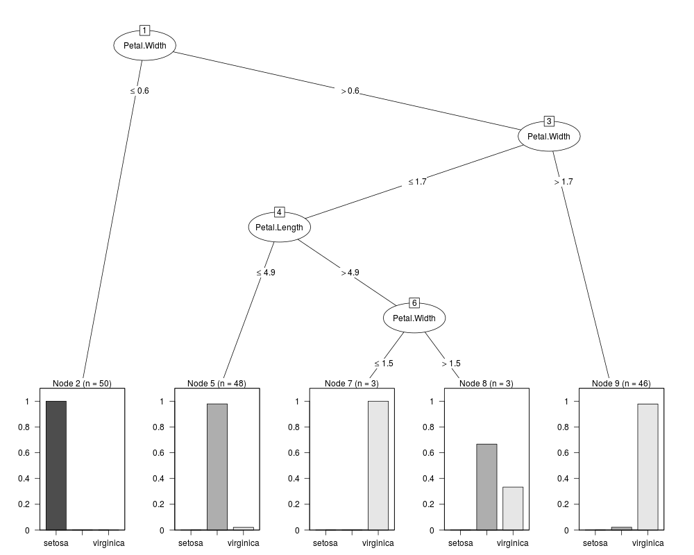
m1 <- J48(Species ~ ., data = iris)
## print and summary
m1
summary(m1) # calls evaluate_Weka_classifier()
table(iris$Species, predict(m1)) # by hand
## visualization
## use partykit package
if(require("partykit", quietly = TRUE)) plot(m1)
## or Graphviz
write_to_dot(m1)
## or Rgraphviz
## Not run:
library("Rgraphviz")
ff <- tempfile()
write_to_dot(m1, ff)
plot(agread(ff))
## End(Not run)
## Using some Weka data sets ...
## J48
DF2 <- read.arff(system.file("arff", "contact-lenses.arff",
package = "RWeka"))
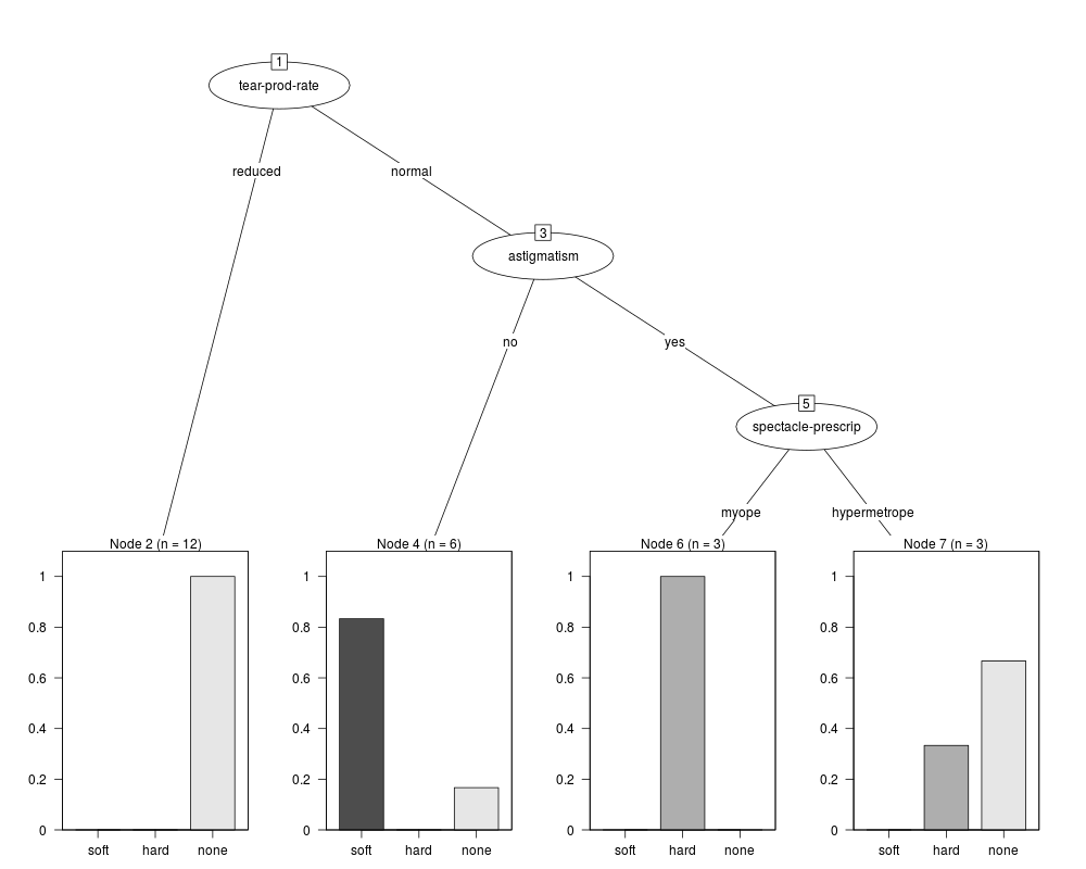
m2 <- J48(`contact-lenses` ~ ., data = DF2)
m2
table(DF2$`contact-lenses`, predict(m2))
if(require("partykit", quietly = TRUE)) plot(m2)
## M5P
DF3 <- read.arff(system.file("arff", "cpu.arff", package = "RWeka"))
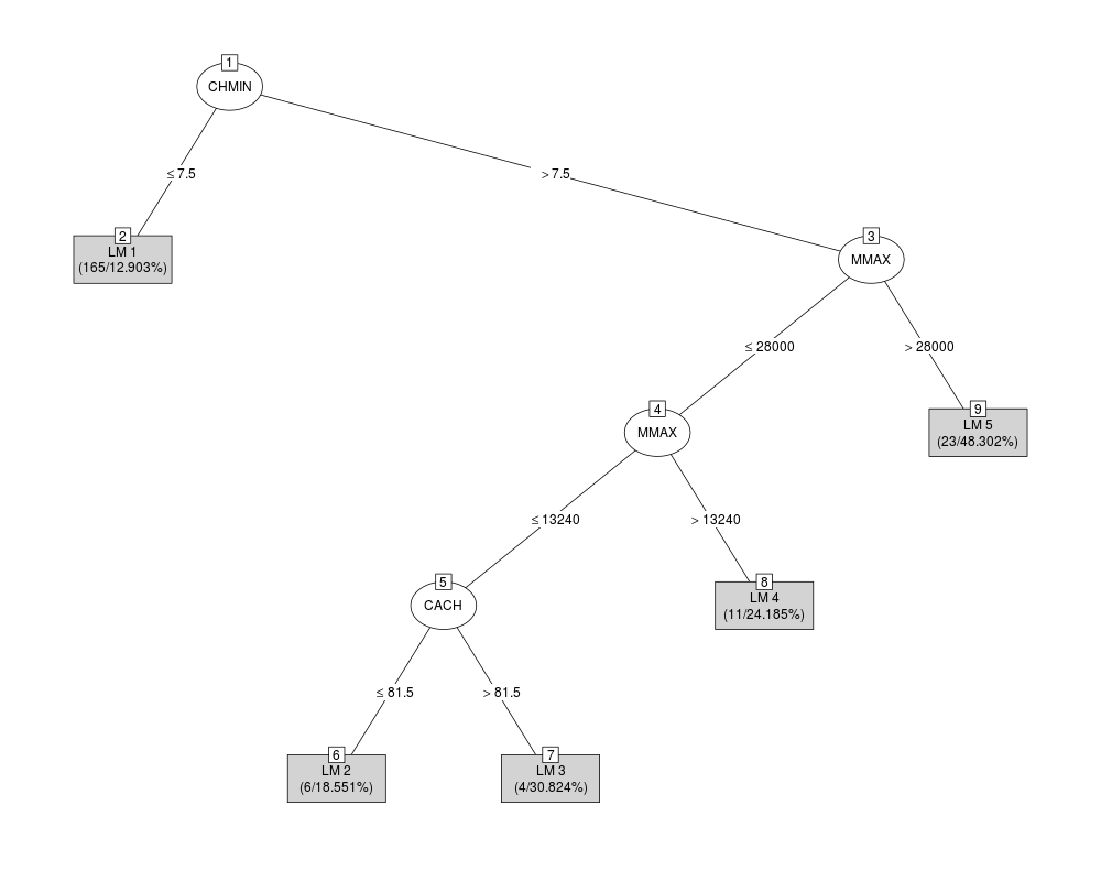
m3 <- M5P(class ~ ., data = DF3)
m3
if(require("partykit", quietly = TRUE)) plot(m3)
## Logistic Model Tree.
DF4 <- read.arff(system.file("arff", "weather.arff", package = "RWeka"))
m4 <- LMT(play ~ ., data = DF4)
m4
table(DF4$play, predict(m4))
## Larger scale example.
if(require("mlbench", quietly = TRUE)
&& require("partykit", quietly = TRUE)) {
## Predict diabetes status for Pima Indian women
data("PimaIndiansDiabetes", package = "mlbench")
## Fit J48 tree with reduced error pruning
m5 <- J48(diabetes ~ ., data = PimaIndiansDiabetes,
control = Weka_control(R = TRUE))
plot(m5)
## (Make sure that the plotting device is big enough for the tree.)
}
Results
R version 3.3.1 (2016-06-21) -- "Bug in Your Hair"
Copyright (C) 2016 The R Foundation for Statistical Computing
Platform: x86_64-pc-linux-gnu (64-bit)

R is free software and comes with ABSOLUTELY NO WARRANTY.
You are welcome to redistribute it under certain conditions.
Type 'license()' or 'licence()' for distribution details.

R is a collaborative project with many contributors.
Type 'contributors()' for more information and
'citation()' on how to cite R or R packages in publications.

Type 'demo()' for some demos, 'help()' for on-line help, or
'help.start()' for an HTML browser interface to help.
Type 'q()' to quit R.

> library(RWeka)
> png(filename="/home/ddbj/snapshot/RGM3/R_CC/result/RWeka/Weka_classifier_trees.Rd_%03d_medium.png", width=480, height=480)
> ### Name: Weka_classifier_trees
> ### Title: R/Weka Classifier Trees
> ### Aliases: Weka_classifier_trees J48 LMT M5P DecisionStump plot.Weka_tree
> ###   parse_Weka_digraph
> ### Keywords: models regression classif tree
>
> ### ** Examples
>
> m1 <- J48(Species ~ ., data = iris)
>
> ## print and summary
> m1
J48 pruned tree
------------------

Petal.Width <= 0.6: setosa (50.0)
Petal.Width > 0.6
|   Petal.Width <= 1.7
|   |   Petal.Length <= 4.9: versicolor (48.0/1.0)
|   |   Petal.Length > 4.9
|   |   |   Petal.Width <= 1.5: virginica (3.0)
|   |   |   Petal.Width > 1.5: versicolor (3.0/1.0)
|   Petal.Width > 1.7: virginica (46.0/1.0)

Number of Leaves  : 	5

Size of the tree : 	9

> summary(m1) # calls evaluate_Weka_classifier()

=== Summary ===

Correctly Classified Instances         147               98      %
Incorrectly Classified Instances         3                2      %
Kappa statistic                          0.97
Mean absolute error                      0.0233
Root mean squared error                  0.108
Relative absolute error                  5.2482 %
Root relative squared error             22.9089 %
Total Number of Instances              150

=== Confusion Matrix ===

  a  b  c   <-- classified as
 50  0  0 |  a = setosa
  0 49  1 |  b = versicolor
  0  2 48 |  c = virginica
> table(iris$Species, predict(m1)) # by hand

             setosa versicolor virginica
  setosa         50          0         0
  versicolor      0         49         1
  virginica       0          2        48
>
> ## visualization
> ## use partykit package
> if(require("partykit", quietly = TRUE)) plot(m1)
> ## or Graphviz
> write_to_dot(m1)
digraph J48Tree {
N0 [label="Petal.Width" ]
N0->N1 [label="<= 0.6"]
N1 [label="setosa (50.0)" shape=box style=filled ]
N0->N2 [label="> 0.6"]
N2 [label="Petal.Width" ]
N2->N3 [label="<= 1.7"]
N3 [label="Petal.Length" ]
N3->N4 [label="<= 4.9"]
N4 [label="versicolor (48.0/1.0)" shape=box style=filled ]
N3->N5 [label="> 4.9"]
N5 [label="Petal.Width" ]
N5->N6 [label="<= 1.5"]
N6 [label="virginica (3.0)" shape=box style=filled ]
N5->N7 [label="> 1.5"]
N7 [label="versicolor (3.0/1.0)" shape=box style=filled ]
N2->N8 [label="> 1.7"]
N8 [label="virginica (46.0/1.0)" shape=box style=filled ]
}

> ## or Rgraphviz
> ## Not run:
> ##D library("Rgraphviz")
> ##D ff <- tempfile()
> ##D write_to_dot(m1, ff)
> ##D plot(agread(ff))
> ## End(Not run)
>
> ## Using some Weka data sets ...
>
> ## J48
> DF2 <- read.arff(system.file("arff", "contact-lenses.arff",
+                              package = "RWeka"))
> m2 <- J48(`contact-lenses` ~ ., data = DF2)
> m2
J48 pruned tree
------------------

tear-prod-rate = reduced: none (12.0)
tear-prod-rate = normal
|   astigmatism = no: soft (6.0/1.0)
|   astigmatism = yes
|   |   spectacle-prescrip = myope: hard (3.0)
|   |   spectacle-prescrip = hypermetrope: none (3.0/1.0)

Number of Leaves  : 	4

Size of the tree : 	7

> table(DF2$`contact-lenses`, predict(m2))

       soft hard none
  soft    5    0    0
  hard    0    3    1
  none    1    0   14
> if(require("partykit", quietly = TRUE)) plot(m2)
>
> ## M5P
> DF3 <- read.arff(system.file("arff", "cpu.arff", package = "RWeka"))
> m3 <- M5P(class ~ ., data = DF3)
Jul 05, 2016 12:01:36 AM com.github.fommil.netlib.BLAS <clinit>
WARNING: Failed to load implementation from: com.github.fommil.netlib.NativeSystemBLAS
Jul 05, 2016 12:01:36 AM com.github.fommil.netlib.BLAS <clinit>
WARNING: Failed to load implementation from: com.github.fommil.netlib.NativeRefBLAS
Jul 05, 2016 12:01:36 AM com.github.fommil.netlib.LAPACK <clinit>
WARNING: Failed to load implementation from: com.github.fommil.netlib.NativeSystemLAPACK
Jul 05, 2016 12:01:36 AM com.github.fommil.netlib.LAPACK <clinit>
WARNING: Failed to load implementation from: com.github.fommil.netlib.NativeRefLAPACK
> m3
M5 pruned model tree:
(using smoothed linear models)

CHMIN <= 7.5 : LM1 (165/12.903%)
CHMIN >  7.5 :
|   MMAX <= 28000 :
|   |   MMAX <= 13240 :
|   |   |   CACH <= 81.5 : LM2 (6/18.551%)
|   |   |   CACH >  81.5 : LM3 (4/30.824%)
|   |   MMAX >  13240 : LM4 (11/24.185%)
|   MMAX >  28000 : LM5 (23/48.302%)

LM num: 1
class =
	-0.0055 * MYCT
	+ 0.0013 * MMIN
	+ 0.0029 * MMAX
	+ 0.8007 * CACH
	+ 0.4015 * CHMAX
	+ 11.0971

LM num: 2
class =
	-1.0307 * MYCT
	+ 0.0086 * MMIN
	+ 0.0031 * MMAX
	+ 0.7866 * CACH
	- 2.4503 * CHMIN
	+ 1.1597 * CHMAX
	+ 70.8672

LM num: 3
class =
	-1.1057 * MYCT
	+ 0.0086 * MMIN
	+ 0.0031 * MMAX
	+ 0.7995 * CACH
	- 2.4503 * CHMIN
	+ 1.1597 * CHMAX
	+ 83.0016

LM num: 4
class =
	-0.8813 * MYCT
	+ 0.0086 * MMIN
	+ 0.0031 * MMAX
	+ 0.6547 * CACH
	- 2.3561 * CHMIN
	+ 1.1597 * CHMAX
	+ 82.5725

LM num: 5
class =
	-0.4882 * MYCT
	+ 0.0218 * MMIN
	+ 0.003 * MMAX
	+ 0.3865 * CACH
	- 1.3252 * CHMIN
	+ 3.3671 * CHMAX
	- 51.8474

Number of Rules : 5
> if(require("partykit", quietly = TRUE)) plot(m3)
>
> ## Logistic Model Tree.
> DF4 <- read.arff(system.file("arff", "weather.arff", package = "RWeka"))
> m4 <- LMT(play ~ ., data = DF4)
> m4
Logistic model tree
------------------
: LM_1:11/11 (14)

Number of Leaves  : 	1

Size of the Tree : 	1
LM_1:
Class 0 :
6.95 +
[outlook=sunny] * -0.65 +
[outlook=overcast] * 2.82 +
[temperature] * -0.02 +
[humidity] * -0.06 +
[windy=TRUE] * -1.38

Class 1 :
-6.95 +
[outlook=sunny] * 0.65 +
[outlook=overcast] * -2.82 +
[temperature] * 0.02 +
[humidity] * 0.06 +
[windy=TRUE] * 1.38

> table(DF4$play, predict(m4))

      yes no
  yes   8  1
  no    1  4
>
> ## Larger scale example.
> if(require("mlbench", quietly = TRUE)
+    && require("partykit", quietly = TRUE)) {
+     ## Predict diabetes status for Pima Indian women
+     data("PimaIndiansDiabetes", package = "mlbench")
+     ## Fit J48 tree with reduced error pruning
+     m5 <- J48(diabetes ~ ., data = PimaIndiansDiabetes,
+               control = Weka_control(R = TRUE))
+     plot(m5)
+     ## (Make sure that the plotting device is big enough for the tree.)
+ }
>
>
>
>
>
> dev.off()
null device
          1
>
|