Draws a SKEW-T, log p axis.

Description

Draws a SKEW-T, log p axis. This is the standard axis for interpreting atmospheric sounding profiles like those collected by the instrument carried aloft by a weather balloon (radiosonde). Use skewt.lines or skewt.points to layer information on top of the skewt axis.

Usage

skewt.axis(BROWN="brown", GREEN="green", redo=FALSE, ... )

Arguments

Details

Radiosondes record temperature, humidity and winds. They can be lifted by weather balloons, dropped from aircraft, there is even something called a glidersonde. The data collected by radiosondes are plotted versus pressure/height to give details on the vertical structure of the atmosphere. The type of plot is called a SKEW-T, log p diagram.
‘skewt.axis’ creates the traditional axis for a SKEW-T, log p diagram, including moist and dry adiabats, etc ...
Generating the necessary plot data is time-consuming, so there is an option to read from a specific dataset that Doug will change.

Value

Returns the par()$plt values, which are used by plotsonde if you choose to plot the wind profile adjacent to the skewt axis.

Author(s)

Doug Nychka

See Also

getsonde, plotsonde, skewt.lines, skewt.points

Examples

# draw a background, then
#    draw the temperature (with a solid line) in color 6
#    draw the dewpoint in color 7
#    overlay the temperature observations in a different color
#    you get the point ...
#
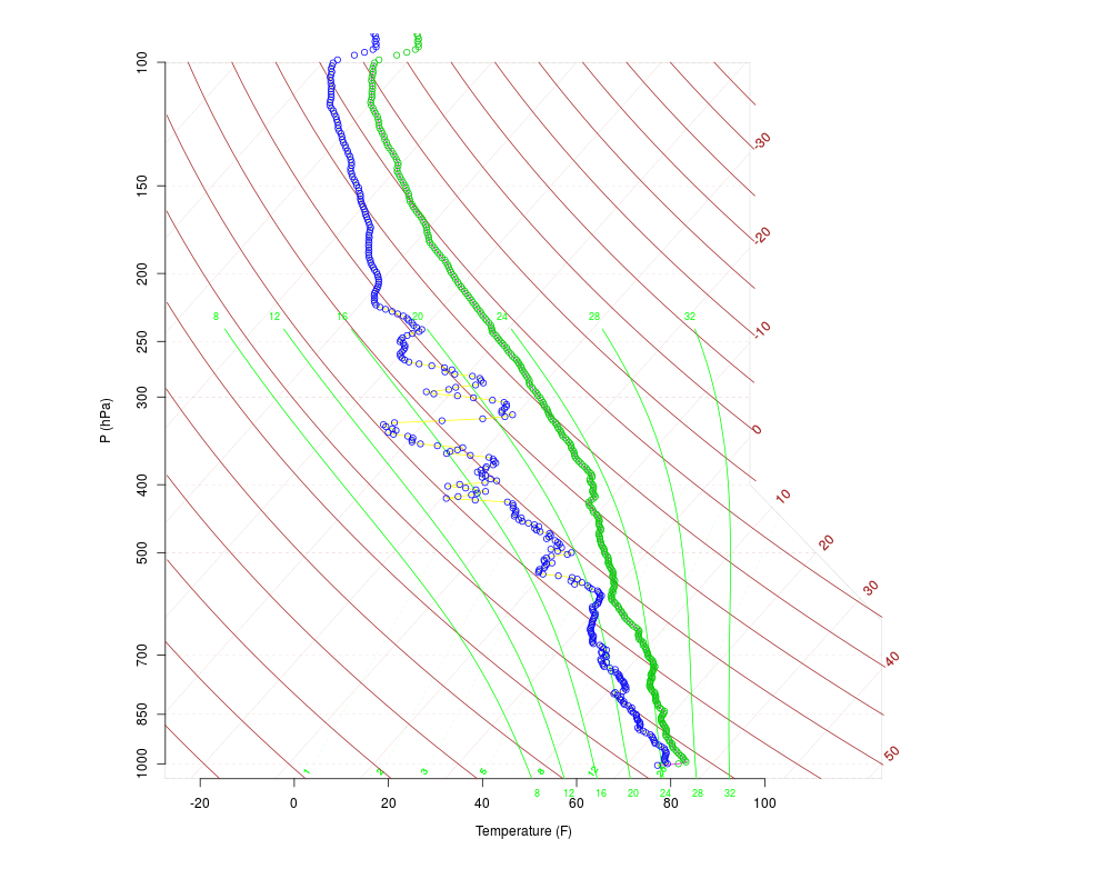
data(ExampleSonde)
skewt.axis( mar=c(5.1, 1.1, 2.1, 5.1) )
skewt.lines( ExampleSonde$temp,  ExampleSonde$press, col = 6)
skewt.lines( ExampleSonde$dewpt, ExampleSonde$press, col = 7)
skewt.points(ExampleSonde$temp,  ExampleSonde$press, col = 3)
skewt.points(ExampleSonde$dewpt, ExampleSonde$press, col = 4)
#
# Changing the moist adiabats: you must edit the code{skewt.axis} function
# directly and then capture the output in code{skewt.data} to be used in 
# subsequent calls.
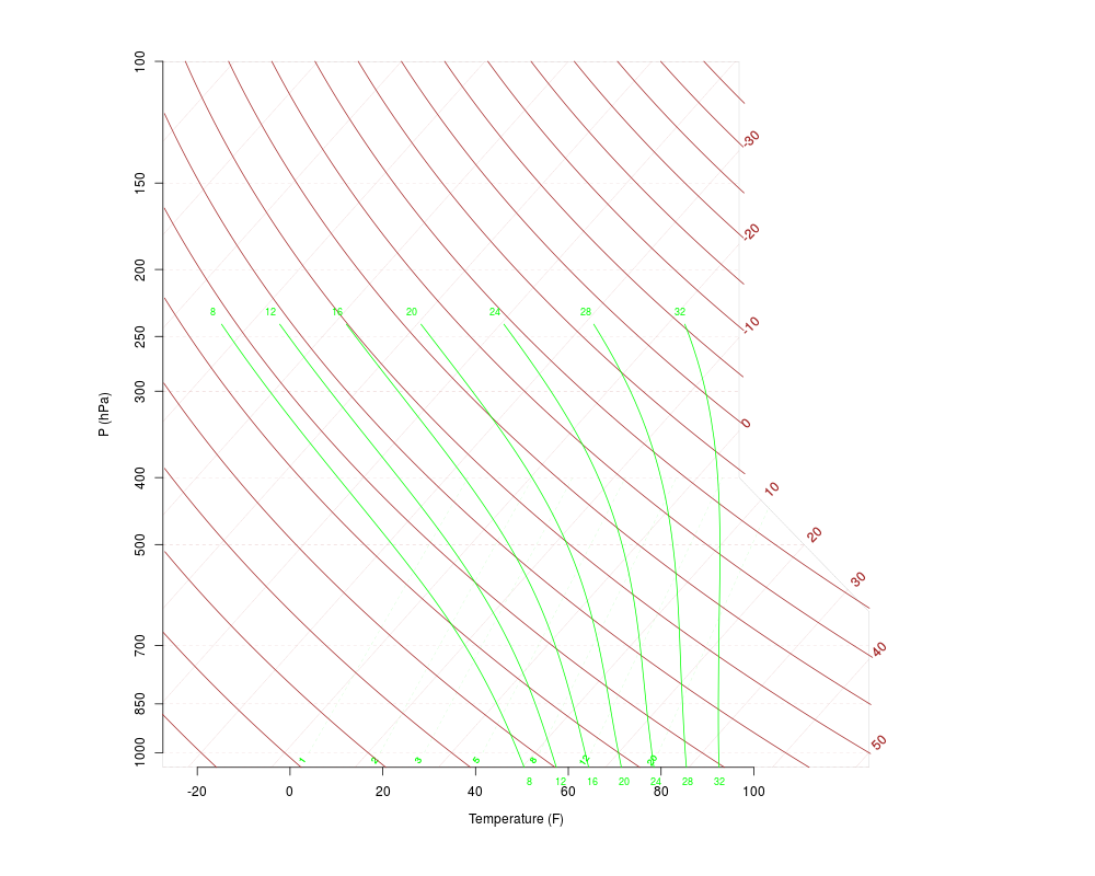
skewt.data <- skewt.axis(redo=TRUE)
skewt.axis() 
skewt.axis() 

Results

R version 3.3.1 (2016-06-21) -- "Bug in Your Hair"
Copyright (C) 2016 The R Foundation for Statistical Computing
Platform: x86_64-pc-linux-gnu (64-bit)

R is free software and comes with ABSOLUTELY NO WARRANTY.
You are welcome to redistribute it under certain conditions.
Type 'license()' or 'licence()' for distribution details.

R is a collaborative project with many contributors.
Type 'contributors()' for more information and
'citation()' on how to cite R or R packages in publications.

Type 'demo()' for some demos, 'help()' for on-line help, or
'help.start()' for an HTML browser interface to help.
Type 'q()' to quit R.

> library(RadioSonde)
> png(filename="/home/ddbj/snapshot/RGM3/R_CC/result/RadioSonde/skewt.axis.Rd_%03d_medium.png", width=480, height=480)
> ### Name: skewt.axis
> ### Title: Draws a SKEW-T, log p axis.
> ### Aliases: skewt.axis
> ### Keywords: hplot
> 
> ### ** Examples
> 
> # draw a background, then
> #    draw the temperature (with a solid line) in color 6
> #    draw the dewpoint in color 7
> #    overlay the temperature observations in a different color
> #    you get the point ...
> #
> data(ExampleSonde)
> skewt.axis( mar=c(5.1, 1.1, 2.1, 5.1) )
> skewt.lines( ExampleSonde$temp,  ExampleSonde$press, col = 6)
> skewt.lines( ExampleSonde$dewpt, ExampleSonde$press, col = 7)
> skewt.points(ExampleSonde$temp,  ExampleSonde$press, col = 3)
> skewt.points(ExampleSonde$dewpt, ExampleSonde$press, col = 4)
> #
> # Changing the moist adiabats: you must edit the code{skewt.axis} function
> # directly and then capture the output in code{skewt.data} to be used in 
> # subsequent calls.
> skewt.data <- skewt.axis(redo=TRUE)
> skewt.axis() 
> skewt.axis() 
> 
> 
> 
> 
> 
> dev.off()
null device 
          1 
>