R Graphical Manual

Browse All

Last data update: 2014.03.03

R: Rearrangement

rearrangement

R Documentation

Rearrangement

Description

Monotonize a step function by rearrangement. Returns a matrix or array of points which are monotonic, or a monotonic function performing linear (or constant) interpolation.

Usage

rearrangement(x,y,n=1000,stochastic=FALSE,avg=TRUE,order=1:length(x))

Arguments

`x`	a list or data frame, the entries of which are vectors containing the x values corresponding to the fitted y values
`y`	a vector, matrix, or three-dimensional array containing the fitted values of a model, typically the result of a regression
`n`	an integer denoting the number of sample points desired
`stochastic`	logical. If TRUE, stochastic sampling will be used
`avg`	logical. If TRUE, the average rearrangement will be computed and outputted
`order`	a vector containing the desired permutation of the elements of 1:length(x). The rearrangement will be performed in the order specified if avg= FALSE, otherwise all the possible orderings are computed and the average rearrangement is reported

Details

This function applies this rearrangement operator of Hardy, Littlewood, and Polya (1952) to the estimate of a monotone function.

Note: rearrangement currently only operates on univariate, bivariate, and trivariate regressions (that is, length(x)<=3).

Value

rearrangement returns a matrix or array of equivalent dimension and size to y that is monotonically increasing in all of its dimensions.

Author(s)

Wesley Graybill, Mingli Chen, Victor Chernozhukov, Ivan Fernandez-Val, Alfred Galichon

References

Chernozhukov, V., I. Fernandez-Val, and a. Galichon. 2009. Improving point and interval estimators of monotone functions by rearrangement. Biometrika 96 (3): 559-575.

Chernozhukov, V., I. Fernandez-Val, and a. Galichon. 2010. Quantile and Probability Curves Without Crossing. Econometrica 78(3): 1093-1125.

Hardy, G.H., J.E. Littlewood, and G. Polya, Inequalities,2nd ed, Cambridge U. Press,1952

Examples

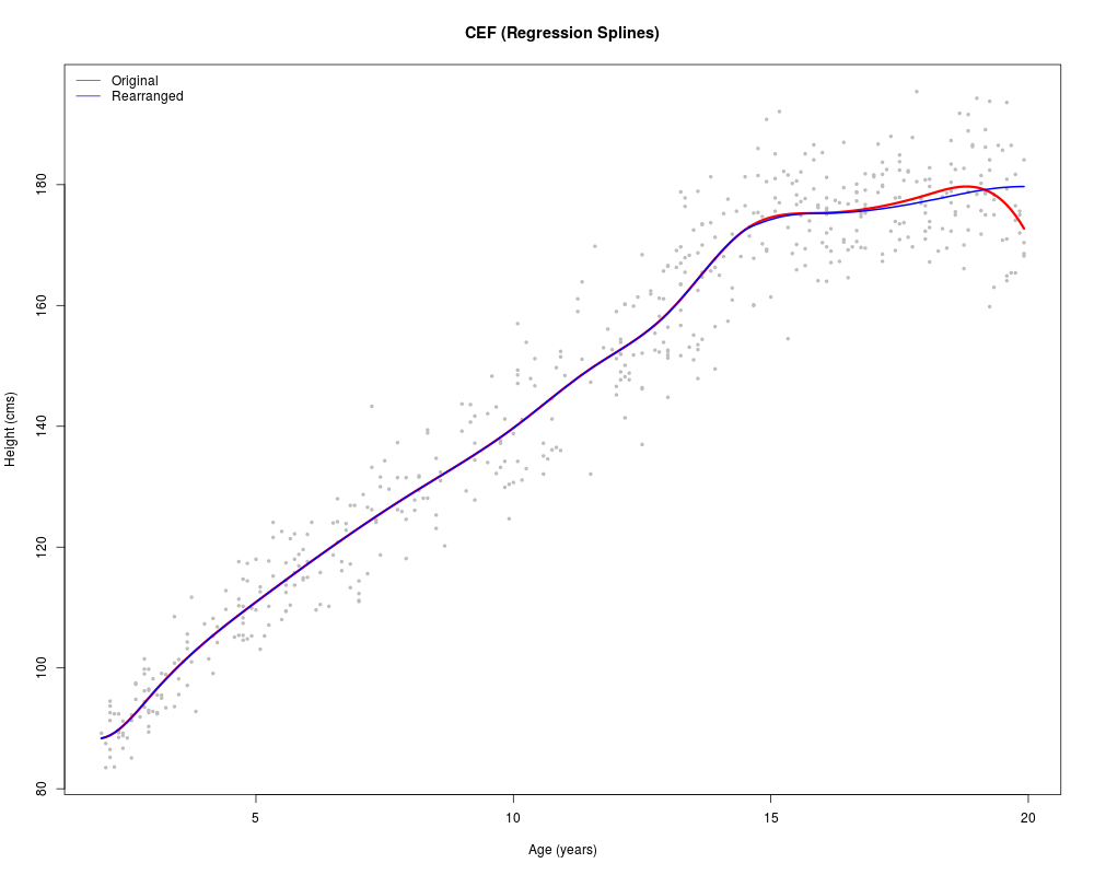
##Univariate example:
library(splines)
data(GrowthChart)
attach(GrowthChart)

ages <- unique(sort(age))
aknots <- c(3, 5, 8, 10, 11.5, 13, 14.5, 16, 18)
splines_age <- bs(age,kn=aknots)
sformula <- height~splines_age
sfunc <- approxfun(age,lm(sformula)$fitted.values)
splreg <- sfunc(ages)
rsplreg <- rearrangement(list(ages),splreg)
plot(age,height,pch=21,bg='gray',cex=.5,xlab="Age (years)",ylab="Height (cms)",
     main="CEF (Regression Splines)",col='gray')
lines(ages,splreg,col='red',lwd=3)
lines(ages,rsplreg,col='blue',lwd=2)
legend("topleft",c('Original','Rearranged'),lty=1,col=c('red','blue'),bty='n')
detach(GrowthChart)

##Bivariate example:
## Not run: library(quantreg)
data(GrowthChart)
attach(GrowthChart)

ages <- unique(sort(age))
taus <- c(1:999)/1000
nage <- 2 * pi * (age - min(age)) / (max(age) - min(age))
nages <- 2 * pi * (ages - min(ages)) / (max(ages) - min(ages))
fform <- height ~ I(sin(nage))+I(cos(nage))+I(sin(2*nage))+I(cos(2*nage))+
          I(sin(3*nage))+I(cos(3*nage))+I(sin(4*nage))+I(cos(4*nage))
ffit <- rq(fform, tau = taus)
fcoefs <- t(ffit$coef)
freg <- rbind(1, sin(nages), cos(nages), sin(2*nages), 
              cos(2*nages),sin(3*nages), cos(3*nages), sin(4*nages), cos(4*nages) )
fcqf <- crossprod(t(fcoefs),freg)
rrfcqf <- rearrangement(list(taus,ages),fcqf, avg=TRUE)
tdom <-c(1,10*c(1:99),999)
adom <-c(1,5*c(1:floor(length(ages)/5)), length(ages))

par(mfrow=c(2,1))
persp(taus[tdom],ages[adom],rrfcqf[tdom,adom],xlab='quantile',
      ylab='age',zlab='height',col='lightgreen',theta=315,phi=25,shade=.5)
title("CQP: Average Quantile/Age Rearrangement")
contour(taus,ages,rrfcqf,xlab='quantile',ylab='age',col='green',
        levels=10*c(ceiling(min(fcqf)/10):floor(max(fcqf)/10)))
title("CQP: Contour (RR-Quantile/Age)")

detach(GrowthChart)

## End(Not run)

Results


R version 3.3.1 (2016-06-21) -- "Bug in Your Hair"
Copyright (C) 2016 The R Foundation for Statistical Computing
Platform: x86_64-pc-linux-gnu (64-bit)

R is free software and comes with ABSOLUTELY NO WARRANTY.
You are welcome to redistribute it under certain conditions.
Type 'license()' or 'licence()' for distribution details.

R is a collaborative project with many contributors.
Type 'contributors()' for more information and
'citation()' on how to cite R or R packages in publications.

Type 'demo()' for some demos, 'help()' for on-line help, or
'help.start()' for an HTML browser interface to help.
Type 'q()' to quit R.

> library(Rearrangement)
Loading required package: quantreg
Loading required package: SparseM

Attaching package: 'SparseM'

The following object is masked from 'package:base':

    backsolve

Loading required package: splines
> png(filename="/home/ddbj/snapshot/RGM3/R_CC/result/Rearrangement/rearrangement.Rd_%03d_medium.png", width=480, height=480)
> ### Name: rearrangement
> ### Title: Rearrangement
> ### Aliases: rearrangement
> ### Keywords: optimize manip regression models
> 
> ### ** Examples
> 
> ##Univariate example:
> library(splines)
> data(GrowthChart)
> attach(GrowthChart)
> 
> ages <- unique(sort(age))
> aknots <- c(3, 5, 8, 10, 11.5, 13, 14.5, 16, 18)
> splines_age <- bs(age,kn=aknots)
> sformula <- height~splines_age
> sfunc <- approxfun(age,lm(sformula)$fitted.values)
> splreg <- sfunc(ages)
> rsplreg <- rearrangement(list(ages),splreg)
> plot(age,height,pch=21,bg='gray',cex=.5,xlab="Age (years)",ylab="Height (cms)",
+      main="CEF (Regression Splines)",col='gray')
> lines(ages,splreg,col='red',lwd=3)
> lines(ages,rsplreg,col='blue',lwd=2)
> legend("topleft",c('Original','Rearranged'),lty=1,col=c('red','blue'),bty='n')
> detach(GrowthChart)
> 
> ##Bivariate example:
> ## Not run: 
> ##D library(quantreg)
> ##D data(GrowthChart)
> ##D attach(GrowthChart)
> ##D 
> ##D ages <- unique(sort(age))
> ##D taus <- c(1:999)/1000
> ##D nage <- 2 * pi * (age - min(age)) / (max(age) - min(age))
> ##D nages <- 2 * pi * (ages - min(ages)) / (max(ages) - min(ages))
> ##D fform <- height ~ I(sin(nage))+I(cos(nage))+I(sin(2*nage))+I(cos(2*nage))+
> ##D           I(sin(3*nage))+I(cos(3*nage))+I(sin(4*nage))+I(cos(4*nage))
> ##D ffit <- rq(fform, tau = taus)
> ##D fcoefs <- t(ffit$coef)
> ##D freg <- rbind(1, sin(nages), cos(nages), sin(2*nages), 
> ##D               cos(2*nages),sin(3*nages), cos(3*nages), sin(4*nages), cos(4*nages) )
> ##D fcqf <- crossprod(t(fcoefs),freg)
> ##D rrfcqf <- rearrangement(list(taus,ages),fcqf, avg=TRUE)
> ##D tdom <-c(1,10*c(1:99),999)
> ##D adom <-c(1,5*c(1:floor(length(ages)/5)), length(ages))
> ##D 
> ##D par(mfrow=c(2,1))
> ##D persp(taus[tdom],ages[adom],rrfcqf[tdom,adom],xlab='quantile',
> ##D       ylab='age',zlab='height',col='lightgreen',theta=315,phi=25,shade=.5)
> ##D title("CQP: Average Quantile/Age Rearrangement")
> ##D contour(taus,ages,rrfcqf,xlab='quantile',ylab='age',col='green',
> ##D         levels=10*c(ceiling(min(fcqf)/10):floor(max(fcqf)/10)))
> ##D title("CQP: Contour (RR-Quantile/Age)")
> ##D 
> ##D detach(GrowthChart)
> ## End(Not run)
> 
> 
> 
> 
> 
> dev.off()
null device 
          1 
>