R Graphical Manual

Browse All

Last data update: 2014.03.03

R: The Plot Routine for an Object of the Shape Routine

plotshape

R Documentation

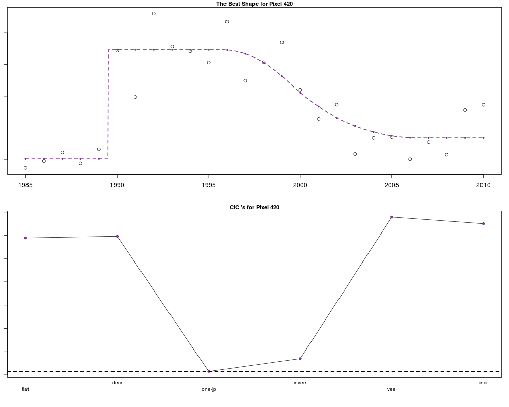
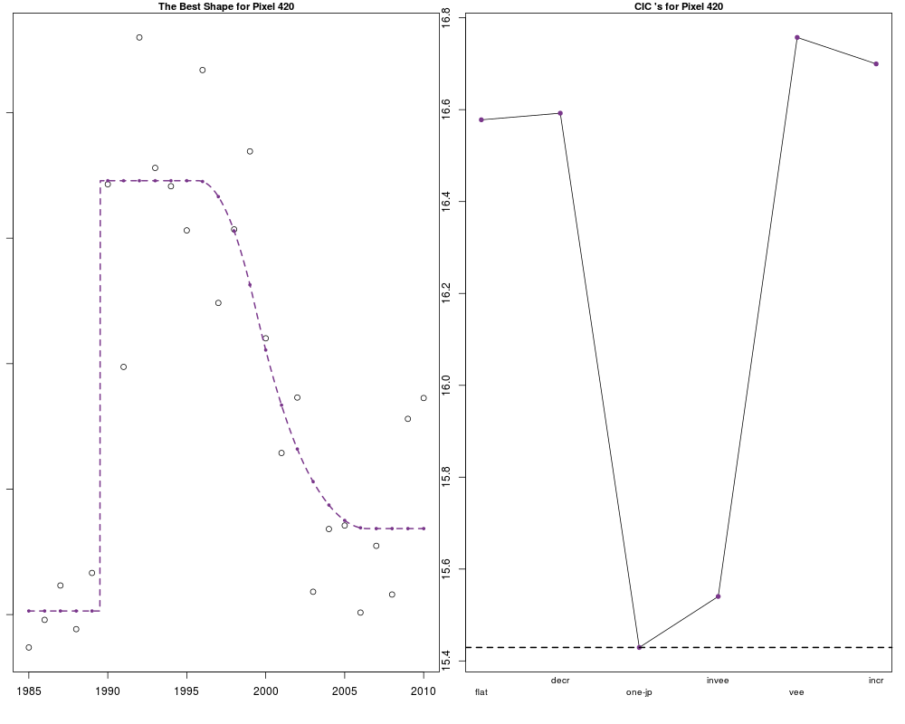
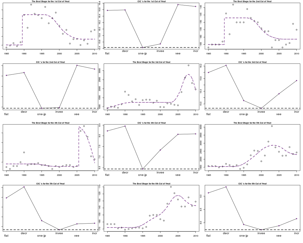
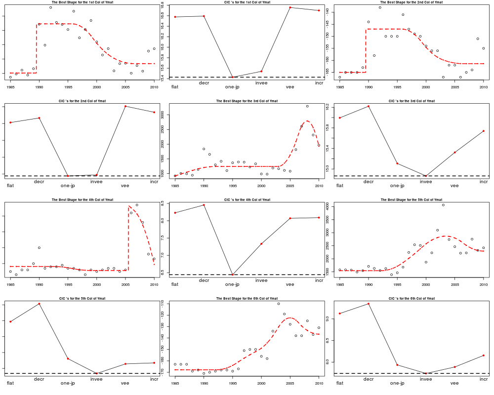
The Plot Routine for an Object of the Shape Routine

Description

This routine can plot the best shape selected by the shape routine for each scatterplot of Landsat signals. It can also plot the "BIC" or "CIC" values against shapes for each scatterplot, which is a way to verify that the best shape selected has the smallest "BIC" or "CIC" value.

Usage

plotshape(object, ids = 1, color = "mediumorchid4", lty = 1, lwd = 1, 
cex = .83, cex.main = .93, form = TRUE, icpic = FALSE, both = TRUE, 
tt = NULL, transpose = FALSE, plot = graphics:::plot)

Arguments

`object`	An object of the shape routine.
`ids`	An integer vector representing a subset of the columns of ymat in the shape routine. Each column of ymat is a time series of Landsat imagery. Suppose that the dimension of ymat is n by k, then each element of "ids" should be an integer between 1 and k. The default is ids = 1.
`color`	The col argument inherited from the plot routine. The default is color = "mediumorchid4".
`lty`	The lty argument inherited from the lines routine. The default is lty = 1.
`lwd`	The lwd argument inherited from the lines routine. The default is lwd = 1.
`cex`	The cex argument inherited from the plot routine. The default is cex = .83.
`cex.main`	The cex.main argument inherited from the par routine. The default is cex.main = .93.
`form`	A logical flag. If it is TRUE, the user will let the plotshape routine to decide the layout of pictures corresponding to the elements in the "ids" vector; otherwise, the user needs to define the layout of pictures before they call the plotshape routine using par(mfrow = ...) or par(mfcol = ...). The default is form = TRUE.
`icpic`	A logical flag. Given an "ids" vector, if it is TRUE, "BIC" or "CIC" values will be plotted against all shapes allowed by the user and the fitted trajectory will not be plotted; otherwise, the fitted trajectory will also be plotted. The default is icpic = FALSE.
`both`	A logical flag. If it is TRUE, then for each element of the "ids" vector, both the fitted trajectory and the "BIC" or "CIC" plot will be made; otherwise, the "BIC" or "CIC" values will not be plotted. The default is both = TRUE.
`tt`	A vector of titles. The user can define its element as a name of the location for a scatterplot, like "Pixel 420". The default is tt = NULL.
`transpose`	A logical flag which can be used only when form is TRUE. If form is TRUE, then the user can transpose the layout the plotshape routine uses to arrange the pictures. For example, the user wants to make 2 pictures, and the default layout of this routine is 2 rows and 1 column. By setting transpose equal to TRUE, the layout will be 1 row and 2 columns. The default is transpose = TRUE.
`plot`	The genetic plot routine in graphics.

Value

A plot showing the fitted trajectory of the best shape, or showing the "BIC" or "CIC" values against shapes of an object of the shape routine.

Author(s)

Xiyue Liao

References

The official documentation for the generic R routine plot: http://stat.ethz.ch/R-manual/R-devel/library/graphics/html/plot.html.

The official documentation for the generic R routine lines: http://stat.ethz.ch/R-manual/R-devel/library/graphics/html/lines.html.

The official documentation for the generic R routine par: http://stat.ethz.ch/R-manual/R-devel/library/graphics/html/par.html.

Examples

	# import the matrix of Landsat signals 
	data("ymat")	

	# define the predictor vector: the year 1985 to the year 2010
	x <- 1985:2010

	# make a fit by the shape routine using "CIC" 
	# and not allow a double jump shape.
	ans <- shape(x, ymat, "CIC", db = FALSE)

	# make a plot for the 1st column of ymat 
	plotshape(ans, ids = 1, both = TRUE, form = TRUE, tt = "Pixel 420")

	# transpose the layout
	plotshape(ans, ids = 1, both = TRUE, form = TRUE, tt = "Pixel 420", transpose = TRUE)

	# make a plot for each of the first 6 columns of ymat 
	# showing the best shape 
	# and "CIC" values against the 7 shapes for each plot.
	par(mfrow = c(3, 2))
	plotshape(ans, ids = 1:6)

	# make a plot for each of the first 6 columns of ymat
	# showing both the best shape
	# and "CIC" values against the 7 shapes for each plot. 		
	# Let the routine make the layout.  
	plotshape(ans, ids = 1:6, form = TRUE, col = 2)

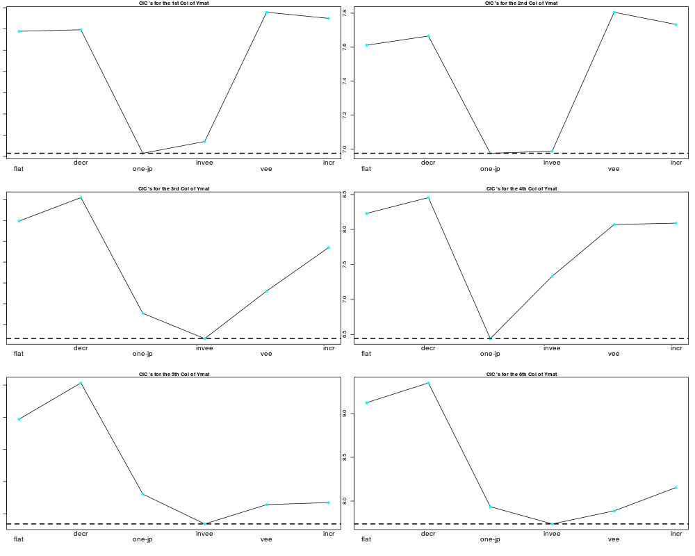
	# plot the ic values only
	plotshape(ans, ids = 1:6, form = TRUE, col = 5, icpic = TRUE)

	# make a title vector
	tts <- paste('Pixel', 1:36, sep = " ")

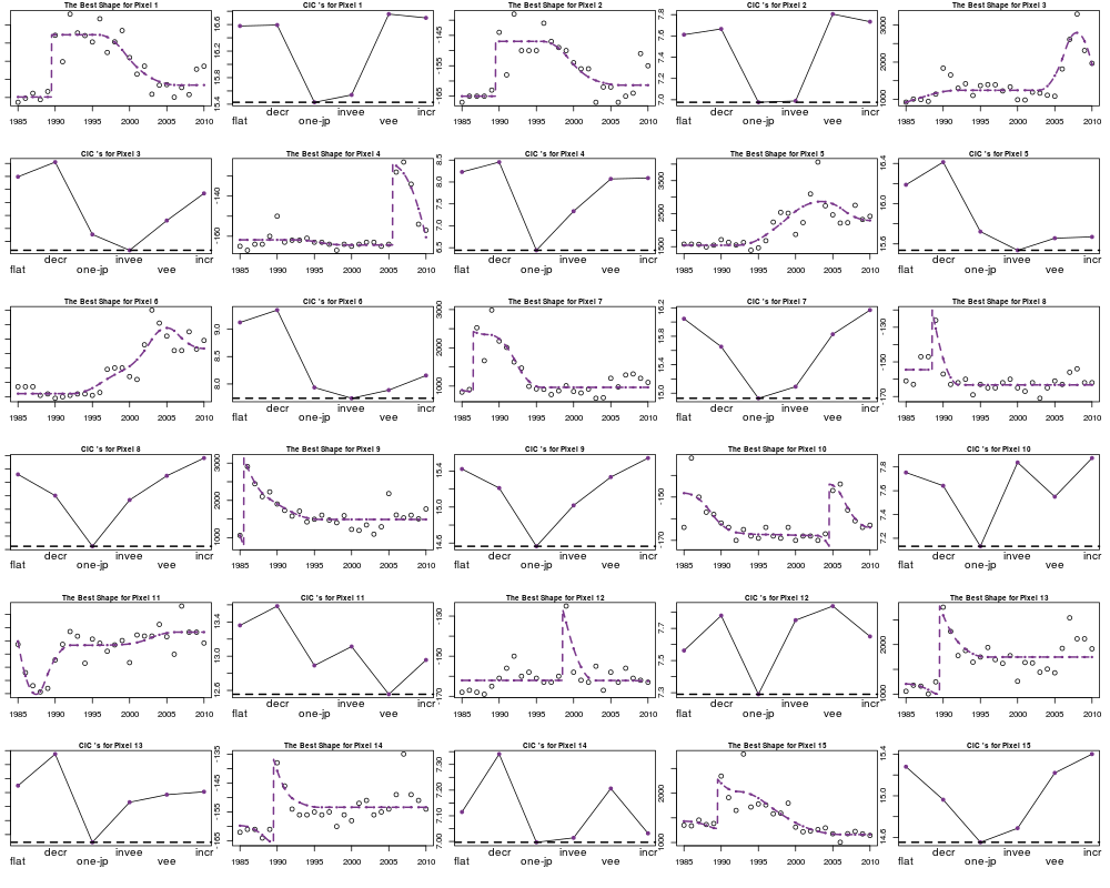
	# make all plots for the 36 scatterplots with the title vector 
	plotshape(ans, ids = 1:15, both = TRUE, form = TRUE, tt = tts[1:15], cex = .5)
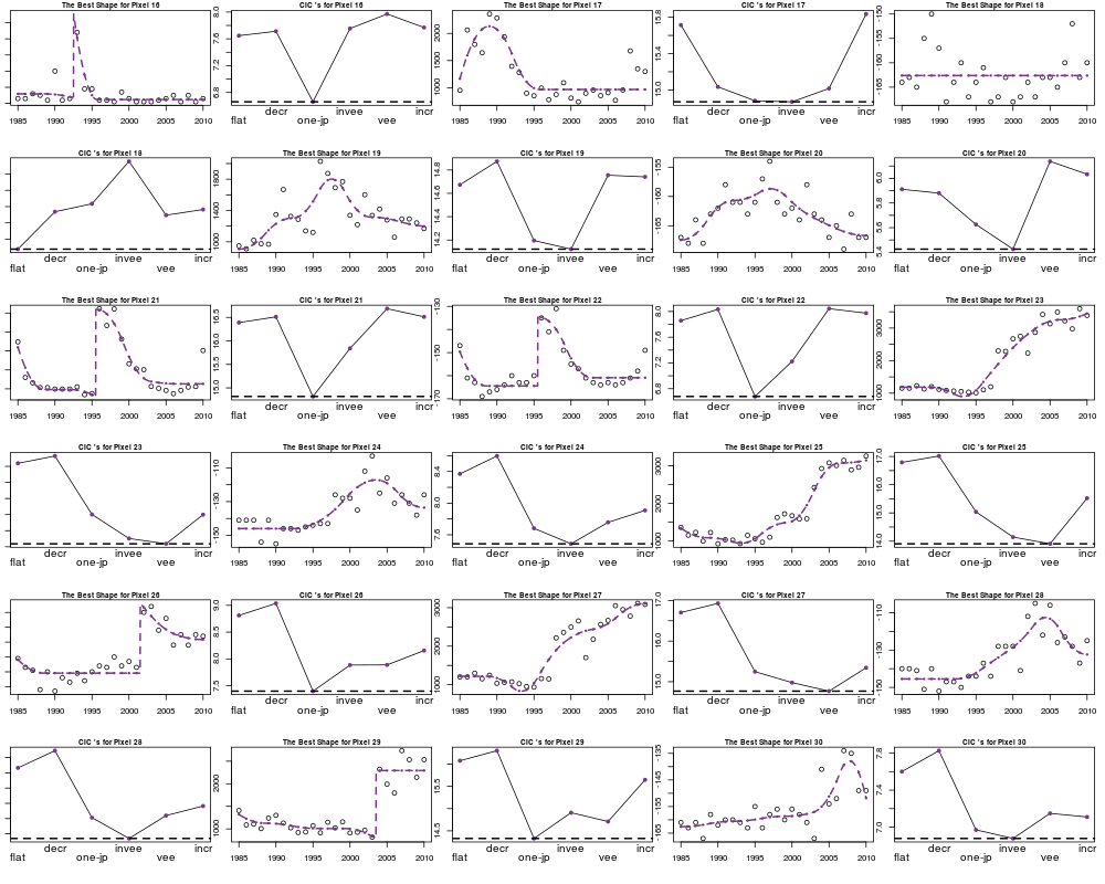
	plotshape(ans, ids = 16:30, both = TRUE, form = TRUE, tt = tts[16:30], lty = 2, cex = .3)
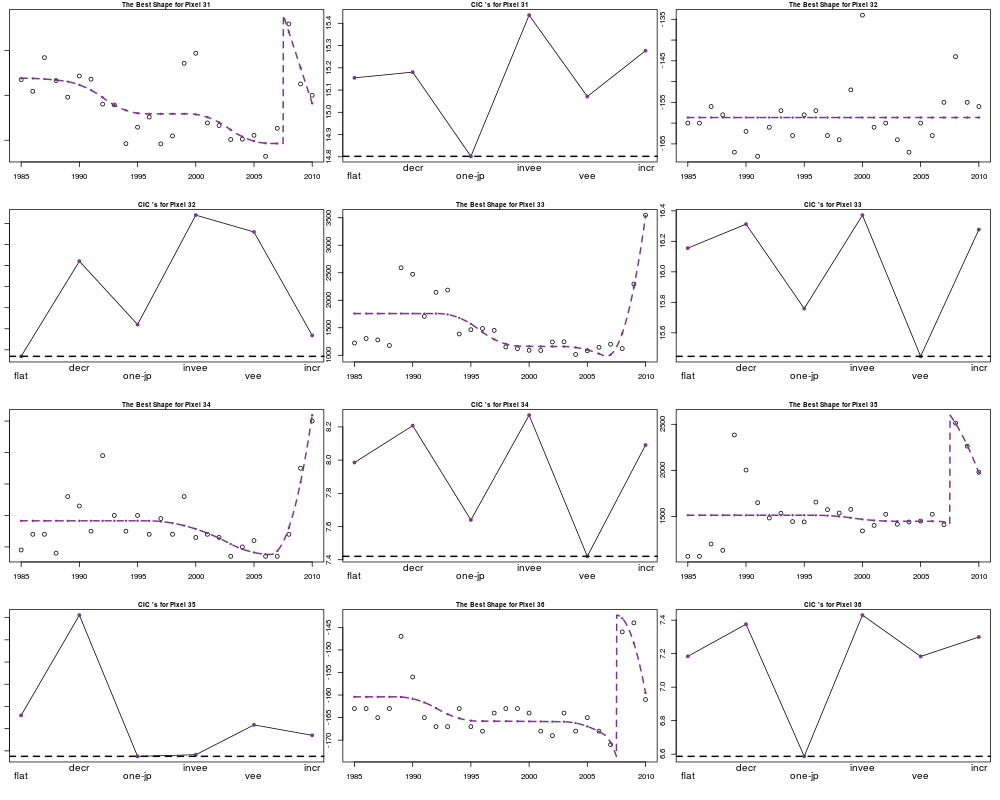
	plotshape(ans, ids = 31:36, both = TRUE, form = TRUE, tt = tts[31:36], lty = 2, cex = .1)

Results


R version 3.3.1 (2016-06-21) -- "Bug in Your Hair"
Copyright (C) 2016 The R Foundation for Statistical Computing
Platform: x86_64-pc-linux-gnu (64-bit)

R is free software and comes with ABSOLUTELY NO WARRANTY.
You are welcome to redistribute it under certain conditions.
Type 'license()' or 'licence()' for distribution details.

R is a collaborative project with many contributors.
Type 'contributors()' for more information and
'citation()' on how to cite R or R packages in publications.

Type 'demo()' for some demos, 'help()' for on-line help, or
'help.start()' for an HTML browser interface to help.
Type 'q()' to quit R.

> library(ShapeSelectForest)
Loading required package: coneproj
Loading required package: raster
Loading required package: sp
Loading required package: rgdal
rgdal: version: 1.1-10, (SVN revision 622)
 Geospatial Data Abstraction Library extensions to R successfully loaded
 Loaded GDAL runtime: GDAL 1.11.3, released 2015/09/16
 Path to GDAL shared files: /usr/share/gdal/1.11
 Loaded PROJ.4 runtime: Rel. 4.9.2, 08 September 2015, [PJ_VERSION: 492]
 Path to PROJ.4 shared files: (autodetected)
 Linking to sp version: 1.2-3 
> png(filename="/home/ddbj/snapshot/RGM3/R_CC/result/ShapeSelectForest/plotshape.Rd_%03d_medium.png", width=480, height=480)
> ### Name: plotshape
> ### Title: The Plot Routine for an Object of the Shape Routine
> ### Aliases: plotshape
> ### Keywords: graphic routine
> 
> ### ** Examples
> 
> 	# import the matrix of Landsat signals 
> 	data("ymat")	
> 
> 	# define the predictor vector: the year 1985 to the year 2010
> 	x <- 1985:2010
> 
> 	# make a fit by the shape routine using "CIC" 
> 	# and not allow a double jump shape.
> 	ans <- shape(x, ymat, "CIC", db = FALSE)
> 
> 	# make a plot for the 1st column of ymat 
> 	plotshape(ans, ids = 1, both = TRUE, form = TRUE, tt = "Pixel 420")
> 
> 	# transpose the layout
> 	plotshape(ans, ids = 1, both = TRUE, form = TRUE, tt = "Pixel 420", transpose = TRUE)
> 
> 	# make a plot for each of the first 6 columns of ymat 
> 	# showing the best shape 
> 	# and "CIC" values against the 7 shapes for each plot.
> 	par(mfrow = c(3, 2))
> 	plotshape(ans, ids = 1:6)
> 
> 	# make a plot for each of the first 6 columns of ymat
> 	# showing both the best shape
> 	# and "CIC" values against the 7 shapes for each plot. 		
> 	# Let the routine make the layout.  
> 	plotshape(ans, ids = 1:6, form = TRUE, col = 2)
> 
> 	# plot the ic values only
> 	plotshape(ans, ids = 1:6, form = TRUE, col = 5, icpic = TRUE)
> 
> 	# make a title vector
> 	tts <- paste('Pixel', 1:36, sep = " ")
> 
> 	# make all plots for the 36 scatterplots with the title vector 
> 	plotshape(ans, ids = 1:15, both = TRUE, form = TRUE, tt = tts[1:15], cex = .5)
> 	plotshape(ans, ids = 16:30, both = TRUE, form = TRUE, tt = tts[16:30], lty = 2, cex = .3)
> 	plotshape(ans, ids = 31:36, both = TRUE, form = TRUE, tt = tts[31:36], lty = 2, cex = .1)
> 
> 
> 
> 
> 
> 
> dev.off()
null device 
          1 
>