R Graphical Manual

Browse All

Last data update: 2014.03.03

R: Hull-White/Vasicek, Ornstein-Uhlenbeck process

HWV	R Documentation

Hull-White/Vasicek, Ornstein-Uhlenbeck process

Description

The (S3) generic function for simulation of Hull-White/Vasicek or gaussian diffusion models, and Ornstein-Uhlenbeck process.

Usage

HWV(N, ...)
OU(N, ...)

## Default S3 method:
HWV(N = 100, M = 1, x0 = 2, t0 = 0, T = 1, Dt, mu = 4, theta = 1,
   sigma = 0.1, ...)
## Default S3 method:
OU(N =100,M=1,x0=2,t0=0,T=1,Dt,mu=4,sigma=0.2, ...)

Arguments

`N`	number of simulation steps.
`M`	number of trajectories.
`x0`	initial value of the process at time code{t0}.
`t0`	initial time.
`T`	final time.
`Dt`	time step of the simulation (discretization). If it is `missing` a default Dt = (T-t0)/N.
`mu`	parameter of the `HWV` and `OU`; see details.
`theta`	parameter of the `HWV`; see details.
`sigma`	the volatility of the `HWV` and `OU`.
`...`	further arguments for (non-default) methods.

Details

The function HWV returns a trajectory of the Hull-White/Vasicek process starting at x0 at time t0; i.e., the diffusion process solution of stochastic differential equation:

dX(t) = mu *( theta- X(t)) dt + sigma dW(t)

The function OU returns a trajectory of the Ornstein-Uhlenbeck starting at x0 at time t0; i.e., the diffusion process solution of stochastic differential equation:

dX(t) = -mu * X(t) dt + sigma dW(t)

Constraints: mu, sigma >0.

Please note that the process is stationary only if mu >0.

Value

`X`	an visible `ts` object.

Author(s)

A.C. Guidoum, K. Boukhetala.

References

Vasicek, O. (1977). An Equilibrium Characterization of the Term Structure. Journal of Financial Economics, 5, 177–188.

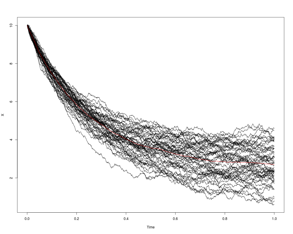
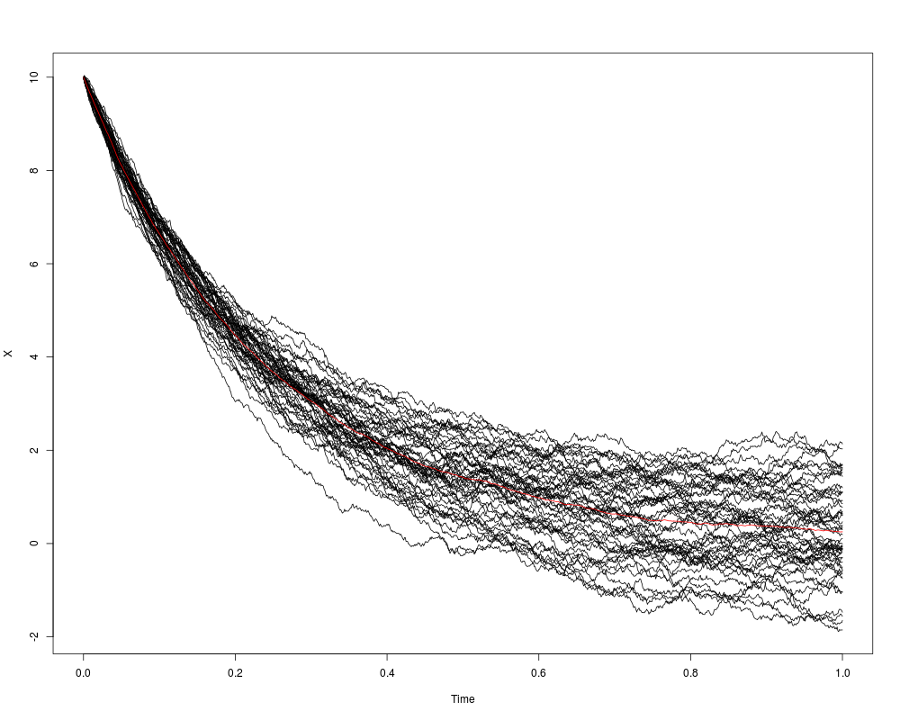
Examples

## Hull-White/Vasicek Models
## dX(t) = 4 * (2.5 - X(t)) * dt + 1 *dW(t), X0=10
set.seed(1234)

X <- HWV(N=1000,M=50,mu = 4, theta = 2.5,sigma = 1,x0=10)
plot(X,plot.type="single")
lines(as.vector(time(X)),rowMeans(X),col="red")

## Ornstein-Uhlenbeck Process
## dX(t) = -4 * X(t) * dt + 1 *dW(t) , X0=2
set.seed(1234)

X <- OU(N=1000,M=50,mu = 4,sigma = 1,x0=10)
plot(X,plot.type="single")
lines(as.vector(time(X)),rowMeans(X),col="red")

Results


R version 3.3.1 (2016-06-21) -- "Bug in Your Hair"
Copyright (C) 2016 The R Foundation for Statistical Computing
Platform: x86_64-pc-linux-gnu (64-bit)

R is free software and comes with ABSOLUTELY NO WARRANTY.
You are welcome to redistribute it under certain conditions.
Type 'license()' or 'licence()' for distribution details.

R is a collaborative project with many contributors.
Type 'contributors()' for more information and
'citation()' on how to cite R or R packages in publications.

Type 'demo()' for some demos, 'help()' for on-line help, or
'help.start()' for an HTML browser interface to help.
Type 'q()' to quit R.

> library(Sim.DiffProc)
Package 'Sim.DiffProc' version 3.2 loaded.
help(Sim.DiffProc) for summary information.
> png(filename="/home/ddbj/snapshot/RGM3/R_CC/result/Sim.DiffProc/HWV.Rd_%03d_medium.png", width=480, height=480)
> ### Name: HWV
> ### Title: Hull-White/Vasicek, Ornstein-Uhlenbeck process
> ### Aliases: HWV OU HWV.default OU.default
> ### Keywords: sde ts
> 
> ### ** Examples
> 
> ## Hull-White/Vasicek Models
> ## dX(t) = 4 * (2.5 - X(t)) * dt + 1 *dW(t), X0=10
> set.seed(1234)
> 
> X <- HWV(N=1000,M=50,mu = 4, theta = 2.5,sigma = 1,x0=10)
> plot(X,plot.type="single")
> lines(as.vector(time(X)),rowMeans(X),col="red")
> 
> ## Ornstein-Uhlenbeck Process
> ## dX(t) = -4 * X(t) * dt + 1 *dW(t) , X0=2
> set.seed(1234)
> 
> X <- OU(N=1000,M=50,mu = 4,sigma = 1,x0=10)
> plot(X,plot.type="single")
> lines(as.vector(time(X)),rowMeans(X),col="red")
> 
> 
> 
> 
> 
> dev.off()
null device 
          1 
>