Simulation of 2-Dim Diffusion Bridge

Description

The (S3) generic function bridgesde2d for simulation of 2-dim diffusion bridge.

Usage

bridgesde2d(N, ...)
## Default S3 method:
bridgesde2d(N = 1000, M = 1, x0 = c(0, 0), y = c(1, 1), t0 = 0, T = 1, Dt, 
   driftx, diffx, drifty, diffy, alpha = 0.5, mu = 0.5, type = c("ito", "str"),
   method = c("euler", "milstein", "predcorr", "smilstein", "taylor", 
   "heun", "rk1", "rk2", "rk3"), ...)
							  
							  
## S3 method for class 'bridgesde2d'
time(x, ...)
## S3 method for class 'bridgesde2d'
mean(x, ...)
## S3 method for class 'bridgesde2d'
median(x, ...)
## S3 method for class 'bridgesde2d'
quantile(x, ...)
## S3 method for class 'bridgesde2d'
kurtosis(x, ...)
## S3 method for class 'bridgesde2d'
skewness(x, ...)
## S3 method for class 'bridgesde2d'
moment(x, order = 2, ...)
## S3 method for class 'bridgesde2d'
bconfint(x, level=0.95, ...)
## S3 method for class 'bridgesde2d'
plot(x, ...)
## S3 method for class 'bridgesde2d'
lines(x, ...)
## S3 method for class 'bridgesde2d'
points(x, ...)	
## S3 method for class 'bridgesde2d'
plot2d(x, ...)
## S3 method for class 'bridgesde2d'
lines2d(x, ...)
## S3 method for class 'bridgesde2d'
points2d(x, ...)								  

Arguments

Details

The function bridgesde2d returns a mts of the diffusion bridge starting at x at time t0 and ending at y at time T.

The methods of approximation are classified according to their different properties. Mainly two criteria of optimality are used in the literature: the strong and the weak (orders of) convergence. The method of simulation can be one among: Euler-Maruyama Order 0.5, Milstein Order 1, Milstein Second-Order, Predictor-Corrector method, Ito-Taylor Order 1.5, Heun Order 2 and Runge-Kutta Order 1, 2 and 3.

For more details see vignette("SDEs").

Value

bridgesde2d returns an object inheriting from class "bridgesde2d".

Author(s)

A.C. Guidoum, K. Boukhetala.

References

Bladt, M. and Sorensen, M. (2007). Simple simulation of diffusion bridges with application to likelihood inference for diffusions. Working Paper, University of Copenhagen.

Iacus, S.M. (2008). Simulation and inference for stochastic differential equations: with R examples. Springer-Verlag, New York

See Also

bridgesde1d for simulation of 1-dim diffusion bridge.

DBridge in package sde.

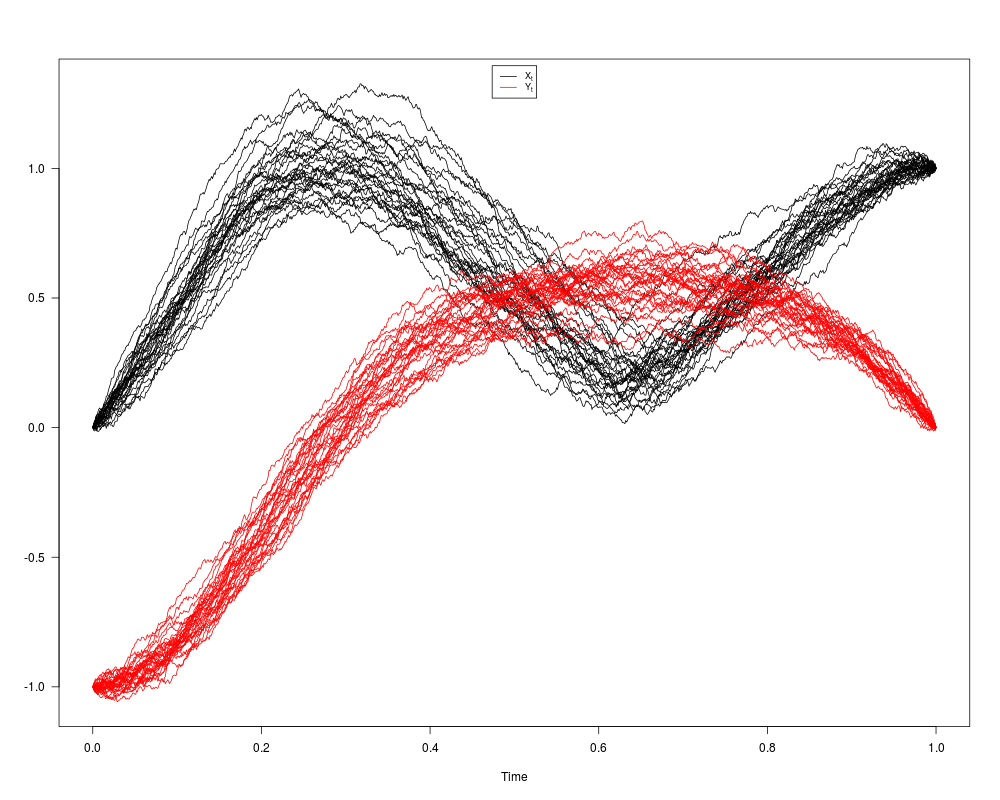
Examples

## dX(t) = 4*(-1-X(t))*Y(t) dt + 0.2 dW1(t)
## dY(t) = 4*(1-Y(t))*X(t) dt + 0.2 dW2(t)
## x01 = 0 , y01 = 1
## x02 = -1, y02 = 0 
## W1(t) and W2(t) two independent Brownian motion
set.seed(1234)

fx <- expression(4*(-1-x)*y)
gx <- expression(0.2)
fy <- expression(4*(1-y)*x)
gy <- expression(0.2)

res <- bridgesde2d(x0=c(0,-1),y=c(1,0),driftx=fx,diffx=gx,drifty=fy,diffy=gy,M=30)
res
plot(res)
dev.new()
plot2d(res,type="n")
points2d(res,col=rgb(0,100,0,50,maxColorValue=255), pch=16)

Results

R version 3.3.1 (2016-06-21) -- "Bug in Your Hair"
Copyright (C) 2016 The R Foundation for Statistical Computing
Platform: x86_64-pc-linux-gnu (64-bit)

R is free software and comes with ABSOLUTELY NO WARRANTY.
You are welcome to redistribute it under certain conditions.
Type 'license()' or 'licence()' for distribution details.

R is a collaborative project with many contributors.
Type 'contributors()' for more information and
'citation()' on how to cite R or R packages in publications.

Type 'demo()' for some demos, 'help()' for on-line help, or
'help.start()' for an HTML browser interface to help.
Type 'q()' to quit R.

> library(Sim.DiffProc)
Package 'Sim.DiffProc' version 3.2 loaded.
help(Sim.DiffProc) for summary information.
> png(filename="/home/ddbj/snapshot/RGM3/R_CC/result/Sim.DiffProc/bridgesde2d.Rd_%03d_medium.png", width=480, height=480)
> ### Name: bridgesde2d
> ### Title: Simulation of 2-Dim Diffusion Bridge
> ### Aliases: bridgesde2d bridgesde2d.default print.bridgesde2d
> ###   time.bridgesde2d mean.bridgesde2d median.bridgesde2d
> ###   quantile.bridgesde2d kurtosis.bridgesde2d skewness.bridgesde2d
> ###   moment.bridgesde2d bconfint.bridgesde2d plot.bridgesde2d
> ###   points.bridgesde2d lines.bridgesde2d plot2d.bridgesde2d
> ###   points2d.bridgesde2d lines2d.bridgesde2d
> ### Keywords: sde ts mts
> 
> ### ** Examples
> 
> ## dX(t) = 4*(-1-X(t))*Y(t) dt + 0.2 dW1(t)
> ## dY(t) = 4*(1-Y(t))*X(t) dt + 0.2 dW2(t)
> ## x01 = 0 , y01 = 1
> ## x02 = -1, y02 = 0 
> ## W1(t) and W2(t) two independent Brownian motion
> set.seed(1234)
> 
> fx <- expression(4*(-1-x)*y)
> gx <- expression(0.2)
> fy <- expression(4*(1-y)*x)
> gy <- expression(0.2)
> 
> res <- bridgesde2d(x0=c(0,-1),y=c(1,0),driftx=fx,diffx=gx,drifty=fy,diffy=gy,M=30)
> res
Ito Bridges Sde 2D:
	| dX(t) = 4 * (-1 - X(t)) * Y(t) * dt + 0.2 * dW1(t)
	| dY(t) = 4 * (1 - Y(t)) * X(t) * dt + 0.2 * dW2(t)
Method:
	| Euler scheme of order 0.5
Summary:
	| Size of process	| N  = 1000.
	| Crossing realized	| (Cx,Cy) = c(30,30).
	| Initial values	| x0 = c(0,-1).
	| Final values		| y  = c(1,0).
	| Time of process	| t in [0,1].
	| Discretization	| Dt = 0.001.
> plot(res)
> dev.new()
Error in dev.new() : no suitable unused file name for pdf()
Execution halted