Supported by Dr. Osamu Ogasawara and  . . |
|
Last data update: 2014.03.03 |
Maximum Pseudo-Likelihood Estimation of 1-Dim SDEDescriptionThe (S3) generic function Usage
fitsde(data, ...)
## Default S3 method:
fitsde(data, drift, diffusion, start = list(), pmle = c("euler","kessler",
   "ozaki", "shoji"), optim.method = "L-BFGS-B",
   lower = -Inf, upper = Inf, ...)

## S3 method for class 'fitsde'
summary(object, ...)
## S3 method for class 'fitsde'
coef(object, ...)
## S3 method for class 'fitsde'
vcov(object, ...)
## S3 method for class 'fitsde'
logLik(object, ...)
## S3 method for class 'fitsde'
AIC(object, ...)
## S3 method for class 'fitsde'
BIC(object, ...)
## S3 method for class 'fitsde'
confint(object,parm, level=0.95, ...)
Arguments
DetailsThe function The For more details see Value
Author(s)A.C. Guidoum, K. Boukhetala. ReferencesKessler, M. (1997). Estimation of an ergodic diffusion from discrete observations. Scand. J. Statist., 24, 211-229. Iacus, S.M. (2008). Simulation and inference for stochastic differential equations: with R examples. Springer-Verlag, New York. Iacus, S.M. (2009). sde: Simulation and Inference for Stochastic Differential Equations. R package version 2.0.10. Iacus, S.M. and all. (2014). The yuima Project: A Computational Framework for Simulation and Inference of Stochastic Differential Equations. Journal of Statistical Software, 57(4). Ozaki, T. (1992). A bridge between nonlinear time series models and nonlinear stochastic dynamical systems: A local linearization approach. Statistica Sinica, 2, 25-83. Shoji, L., Ozaki, T. (1998). Estimation for nonlinear stochastic differential equations by a local linearization method. Stochastic Analysis and Applications, 16, 733-752. Dacunha, D.C. and Florens, D.Z. (1986). Estimation of the Coefficients of a Diffusion from Discrete Observations. Stochastics. 19, 263–284. Dohnal, G. (1987). On estimating the diffusion coefficient. J. Appl.Prob., 24, 105–114. Genon, V.C. (1990). Maximum constrast estimation for diffusion processes from discrete observation. Statistics, 21, 99–116. Nicolau, J. (2004). Introduction to the estimation of stochastic differential equations based on discrete observations. Autumn School and International Conference, Stochastic Finance. Ait-Sahalia, Y. (1999). Transition densities for interest rate and other nonlinear diffusions. The Journal of Finance, 54, 1361–1395. Ait-Sahalia, Y. (2002). Maximum likelihood estimation of discretely sampled diffusions: a closed-form approximation approach. Econometrica. 70, 223–262. B.L.S. Prakasa Rao. (1999). Statistical Inference for Diffusion Type Processes. Arnold, London and Oxford University press, New York. Kutoyants, Y.A. (2004). Statistical Inference for Ergodic Diffusion Processes. Springer, London. See Also
Examples
##### Example 1:
## Modele GBM (BS)
## dX(t) = theta1 * X(t) * dt + theta2 * x * dW(t)
## Simulation of data
set.seed(1234)
X <- GBM(N =1000,theta=4,sigma=1)
## Estimation: true theta=c(4,1)
fx <- expression(theta[1]*x)
gx <- expression(theta[2]*x)
fres <- fitsde(data=X,drift=fx,diffusion=gx,start = list(theta1=1,theta2=1),
lower=c(0,0))
fres
summary(fres)
coef(fres)
logLik(fres)
AIC(fres)
BIC(fres)
vcov(fres)
confint(fres,level=0.95)
##### Example 2:
## Nonlinear mean reversion (Ait-Sahalia) modele
## dX(t) = (theta1 + theta2*x + theta3*x^2) * dt + theta4 * x^theta5 * dW(t)
## Simulation of the process X(t)
set.seed(1234)
f <- expression(1 - 11*x + 2*x^2)
g <- expression(x^0.5)
res <- snssde1d(drift=f,diffusion=g,M=1,N=1000,Dt=0.001,x0=5)
mydata1 <- res$X
## Estimation
## true param theta= c(1,-11,2,1,0.5)
true <- c(1,-11,2,1,0.5)
pmle <- eval(formals(fitsde.default)$pmle)
fx <- expression(theta[1] + theta[2]*x + theta[3]*x^2)
gx <- expression(theta[4]*x^theta[5])
fres <- lapply(1:4, function(i) fitsde(mydata1,drift=fx,diffusion=gx,
pmle=pmle[i],start = list(theta1=1,theta2=1,theta3=1,theta4=1,
theta5=1),optim.method = "L-BFGS-B"))
Coef <- data.frame(true,do.call("cbind",lapply(1:4,function(i) coef(fres[[i]]))))
names(Coef) <- c("True",pmle)
Summary <- data.frame(do.call("rbind",lapply(1:4,function(i) logLik(fres[[i]]))),
do.call("rbind",lapply(1:4,function(i) AIC(fres[[i]]))),
do.call("rbind",lapply(1:4,function(i) BIC(fres[[i]]))),
row.names=pmle)
names(Summary) <- c("logLik","AIC","BIC")
Coef
Summary
##### Example 3:
## dX(t) = (theta1*x*t+theta2*tan(x)) *dt + theta3*t *dW(t)
## Simulation of data
set.seed(1234)
f <- expression(2*x*t-tan(x))
g <- expression(1.25*t)
sim <- snssde1d(drift=f,diffusion=g,M=1,N=1000,Dt=0.001,x0=10)
mydata2 <- sim$X
## Estimation
## true param theta= c(2,-1,1.25)
true <- c(2,-1,1.25)
fx <- expression(theta[1]*x*t+theta[2]*tan(x))
gx <- expression(theta[3]*t)
fres <- lapply(1:4, function(i) fitsde(mydata2,drift=fx,diffusion=gx,
pmle=pmle[i],start = list(theta1=1,theta2=1,theta3=1),
optim.method = "L-BFGS-B"))
Coef <- data.frame(true,do.call("cbind",lapply(1:4,function(i) coef(fres[[i]]))))
names(Coef) <- c("True",pmle)
Summary <- data.frame(do.call("rbind",lapply(1:4,function(i) logLik(fres[[i]]))),
do.call("rbind",lapply(1:4,function(i) AIC(fres[[i]]))),
do.call("rbind",lapply(1:4,function(i) BIC(fres[[i]]))),
row.names=pmle)
names(Summary) <- c("logLik","AIC","BIC")
Coef
Summary
##### Example 4:
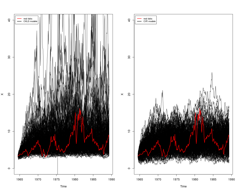
## Application to real data
## CKLS modele vs CIR modele
## CKLS (mod1): dX(t) = (theta1+theta2* X(t))* dt + theta3 * X(t)^theta4 * dW(t)
## CIR (mod2): dX(t) = (theta1+theta2* X(t))* dt + theta3 * sqrt(X(t)) * dW(t)
set.seed(1234)
data(Irates)
rates <- Irates[,"r1"]
rates <- window(rates, start=1964.471, end=1989.333)
fx1 <- expression(theta[1]+theta[2]*x)
gx1 <- expression(theta[3]*x^theta[4])
gx2 <- expression(theta[3]*sqrt(x))
fitmod1 <- fitsde(rates,drift=fx1,diffusion=gx1,pmle="euler",start = list(theta1=1,theta2=1,
theta3=1,theta4=1),optim.method = "L-BFGS-B")
fitmod2 <- fitsde(rates,drift=fx1,diffusion=gx2,pmle="euler",start = list(theta1=1,theta2=1,
theta3=1),optim.method = "L-BFGS-B")
summary(fitmod1)
summary(fitmod2)
coef(fitmod1)
coef(fitmod2)
confint(fitmod1,parm=c('theta2','theta3'))
confint(fitmod2,parm=c('theta2','theta3'))
AIC(fitmod1)
AIC(fitmod2)
## Display
## CKLS Modele
op <- par(mfrow = c(1, 2))
theta <- coef(fitmod1)
N <- length(rates)
res <- snssde1d(drift=fx1,diffusion=gx1,M=200,t0=time(rates)[1],T=time(rates)[N],
Dt=deltat(rates),x0=rates[1],N)
plot(res,plot.type="single",ylim=c(0,40))
lines(rates,col=2,lwd=2)
legend("topleft",c("real data","CKLS modele"),inset = .01,col=c(2,1),lwd=2,cex=0.8)
## CIR Modele
theta <- coef(fitmod2)
res <- snssde1d(drift=fx1,diffusion=gx2,M=200,t0=time(rates)[1],T=time(rates)[N],
Dt=deltat(rates),x0=rates[1],N)
plot(res,plot.type="single",ylim=c(0,40))
lines(rates,col=2,lwd=2)
legend("topleft",c("real data","CIR modele"),inset = .01,col=c(2,1),lwd=2,cex=0.8)
par(op)
Results
R version 3.3.1 (2016-06-21) -- "Bug in Your Hair"
Copyright (C) 2016 The R Foundation for Statistical Computing
Platform: x86_64-pc-linux-gnu (64-bit)

R is free software and comes with ABSOLUTELY NO WARRANTY.
You are welcome to redistribute it under certain conditions.
Type 'license()' or 'licence()' for distribution details.

R is a collaborative project with many contributors.
Type 'contributors()' for more information and
'citation()' on how to cite R or R packages in publications.

Type 'demo()' for some demos, 'help()' for on-line help, or
'help.start()' for an HTML browser interface to help.
Type 'q()' to quit R.

> library(Sim.DiffProc)
Package 'Sim.DiffProc' version 3.2 loaded.
help(Sim.DiffProc) for summary information.
> png(filename="/home/ddbj/snapshot/RGM3/R_CC/result/Sim.DiffProc/fitsde.Rd_%03d_medium.png", width=480, height=480)
> ### Name: fitsde
> ### Title: Maximum Pseudo-Likelihood Estimation of 1-Dim SDE
> ### Aliases: fitsde fitsde.default summary.fitsde print.fitsde vcov.fitsde
> ###   AIC.fitsde BIC.fitsde logLik.fitsde coef.fitsde confint.fitsde
> ### Keywords: fit ts sde
>
> ### ** Examples
>
> #####  Example 1:
>
> ## Modele GBM (BS)
> ## dX(t) = theta1 * X(t) * dt + theta2 * x * dW(t)
> ## Simulation of data
> set.seed(1234)
>
> X <- GBM(N =1000,theta=4,sigma=1)
> ## Estimation: true theta=c(4,1)
> fx <- expression(theta[1]*x)
> gx <- expression(theta[2]*x)
>
> fres <- fitsde(data=X,drift=fx,diffusion=gx,start = list(theta1=1,theta2=1),
+               lower=c(0,0))
> fres

Call:
fitsde(data = X, drift = fx, diffusion = gx, start = list(theta1 = 1,
    theta2 = 1), lower = c(0, 0))

Coefficients:
  theta1   theta2
3.160720 1.000225
> summary(fres)
Pseudo maximum likelihood estimation

Method:  Euler
Call:
fitsde(data = X, drift = fx, diffusion = gx, start = list(theta1 = 1,
    theta2 = 1), lower = c(0, 0))

Coefficients:
       Estimate Std. Error
theta1 3.160720 1.00022484
theta2 1.000225 0.02236563

-2 log L: -1330.008
> coef(fres)
  theta1   theta2
3.160720 1.000225
> logLik(fres)
[1] 665.004
> AIC(fres)
[1] -1326.008
> BIC(fres)
[1] -1316.19
> vcov(fres)
              theta1        theta2
theta1  1.000450e+00 -1.385373e-08
theta2 -1.385373e-08  5.002214e-04
> confint(fres,level=0.95)
          2.5 %   97.5 %
theta1 1.200315 5.121125
theta2 0.956389 1.044061
>
> ## No test:
> #####  Example 2:
>
>
> ## Nonlinear mean reversion (Ait-Sahalia) modele
> ## dX(t) = (theta1 + theta2*x + theta3*x^2) * dt + theta4 * x^theta5 * dW(t)
> ## Simulation of the process X(t)
> set.seed(1234)
>
> f <- expression(1 - 11*x + 2*x^2)
> g <- expression(x^0.5)
> res <- snssde1d(drift=f,diffusion=g,M=1,N=1000,Dt=0.001,x0=5)
> mydata1 <- res$X
>
> ## Estimation
> ## true param theta= c(1,-11,2,1,0.5)
> true <- c(1,-11,2,1,0.5)
> pmle <- eval(formals(fitsde.default)$pmle)
>
> fx <- expression(theta[1] + theta[2]*x + theta[3]*x^2)
> gx <- expression(theta[4]*x^theta[5])
>
> fres <- lapply(1:4, function(i) fitsde(mydata1,drift=fx,diffusion=gx,
+ 	             pmle=pmle[i],start = list(theta1=1,theta2=1,theta3=1,theta4=1,
+                  theta5=1),optim.method = "L-BFGS-B"))
> Coef <- data.frame(true,do.call("cbind",lapply(1:4,function(i) coef(fres[[i]]))))
> names(Coef) <- c("True",pmle)
> Summary <- data.frame(do.call("rbind",lapply(1:4,function(i) logLik(fres[[i]]))),
+                       do.call("rbind",lapply(1:4,function(i) AIC(fres[[i]]))),
+                       do.call("rbind",lapply(1:4,function(i) BIC(fres[[i]]))),
+                       row.names=pmle)
> names(Summary) <- c("logLik","AIC","BIC")
> Coef
        True      euler     kessler       ozaki       shoji
theta1   1.0  0.6873700  0.66607155  0.65115001  0.68374592
theta2 -11.0 -6.9947010 -6.86096214 -6.85205839 -6.92324706
theta3   2.0  0.1152499  0.06059366  0.06270915  0.07623474
theta4   1.0  1.0022594  1.00664000  1.00512419  1.00547899
theta5   0.5  0.5055101  0.50662118  0.50800957  0.50539687
> Summary
          logLik       AIC       BIC
euler   2758.713 -5507.427 -5503.609
kessler 2758.610 -5507.219 -5503.402
ozaki   2758.528 -5507.056 -5503.239
shoji   2758.709 -5507.419 -5503.601
>
>
> #####  Example 3:
>
> ## dX(t) = (theta1*x*t+theta2*tan(x)) *dt + theta3*t *dW(t)
> ## Simulation of data
> set.seed(1234)
>
> f <- expression(2*x*t-tan(x))
> g <- expression(1.25*t)
> sim <- snssde1d(drift=f,diffusion=g,M=1,N=1000,Dt=0.001,x0=10)
> mydata2 <- sim$X
>
> ## Estimation
> ## true param theta= c(2,-1,1.25)
> true <- c(2,-1,1.25)
>
> fx <- expression(theta[1]*x*t+theta[2]*tan(x))
> gx <- expression(theta[3]*t)
>
> fres <- lapply(1:4, function(i) fitsde(mydata2,drift=fx,diffusion=gx,
+ 	             pmle=pmle[i],start = list(theta1=1,theta2=1,theta3=1),
+ 				 optim.method = "L-BFGS-B"))
Warning messages:
1: In log(1 + (A(t0, x0, theta)/(x0 * Ax(t0, x0, theta))) * (exp(Ax(t0,  :
  NaNs produced
2: In log(1 + (A(t0, x0, theta)/(x0 * Ax(t0, x0, theta))) * (exp(Ax(t0,  :
  NaNs produced
3: In log(1 + (A(t0, x0, theta)/(x0 * Ax(t0, x0, theta))) * (exp(Ax(t0,  :
  NaNs produced
4: In log(1 + (A(t0, x0, theta)/(x0 * Ax(t0, x0, theta))) * (exp(Ax(t0,  :
  NaNs produced
5: In log(1 + (A(t0, x0, theta)/(x0 * Ax(t0, x0, theta))) * (exp(Ax(t0,  :
  NaNs produced
6: In log(1 + (A(t0, x0, theta)/(x0 * Ax(t0, x0, theta))) * (exp(Ax(t0,  :
  NaNs produced
7: In log(1 + (A(t0, x0, theta)/(x0 * Ax(t0, x0, theta))) * (exp(Ax(t0,  :
  NaNs produced
> Coef <- data.frame(true,do.call("cbind",lapply(1:4,function(i) coef(fres[[i]]))))
> names(Coef) <- c("True",pmle)
> Summary <- data.frame(do.call("rbind",lapply(1:4,function(i) logLik(fres[[i]]))),
+                       do.call("rbind",lapply(1:4,function(i) AIC(fres[[i]]))),
+                       do.call("rbind",lapply(1:4,function(i) BIC(fres[[i]]))),
+                       row.names=pmle)
> names(Summary) <- c("logLik","AIC","BIC")
> Coef
        True     euler    kessler      ozaki      shoji
theta1  2.00  1.914026 0.95314362  1.9115444  1.9085177
theta2 -1.00 -0.990799 0.01136956 -0.9897514 -0.9612274
theta3  1.25  1.255735 1.64358954  1.2834434  1.3245215
> Summary
          logLik       AIC       BIC
euler   2801.036 -5596.073 -5588.255
kessler 2584.406 -5162.812 -5154.994
ozaki   2778.965 -5551.929 -5544.112
shoji   2793.992 -5581.984 -5574.166
> ## End(No test)
>
> #####  Example 4:
>
> ## Application to real data
> ## CKLS modele vs CIR modele
> ## CKLS (mod1):  dX(t) = (theta1+theta2* X(t))* dt + theta3 * X(t)^theta4 * dW(t)
> ## CIR  (mod2):  dX(t) = (theta1+theta2* X(t))* dt + theta3 * sqrt(X(t))  * dW(t)
> set.seed(1234)
>
> data(Irates)
> rates <- Irates[,"r1"]
> rates <- window(rates, start=1964.471, end=1989.333)
>
> fx1 <- expression(theta[1]+theta[2]*x)
> gx1 <- expression(theta[3]*x^theta[4])
> gx2 <- expression(theta[3]*sqrt(x))
>
> fitmod1 <- fitsde(rates,drift=fx1,diffusion=gx1,pmle="euler",start = list(theta1=1,theta2=1,
+                   theta3=1,theta4=1),optim.method = "L-BFGS-B")
> fitmod2 <- fitsde(rates,drift=fx1,diffusion=gx2,pmle="euler",start = list(theta1=1,theta2=1,
+                   theta3=1),optim.method = "L-BFGS-B")
> summary(fitmod1)
Pseudo maximum likelihood estimation

Method:  Euler
Call:
fitsde(data = rates, drift = fx1, diffusion = gx1, pmle = "euler",
    start = list(theta1 = 1, theta2 = 1, theta3 = 1, theta4 = 1),
    optim.method = "L-BFGS-B")

Coefficients:
         Estimate Std. Error
theta1  2.0769516 0.98838467
theta2 -0.2631871 0.19544290
theta3  0.1302158 0.02523105
theta4  1.4513173 0.10323740

-2 log L: 475.7572
> summary(fitmod2)
Pseudo maximum likelihood estimation

Method:  Euler
Call:
fitsde(data = rates, drift = fx1, diffusion = gx2, pmle = "euler",
    start = list(theta1 = 1, theta2 = 1, theta3 = 1), optim.method = "L-BFGS-B")

Coefficients:
         Estimate Std. Error
theta1  2.6387593 1.18754725
theta2 -0.3606083 0.18896205
theta3  0.8650745 0.03549428

-2 log L: 563.7025
> coef(fitmod1)
    theta1     theta2     theta3     theta4
 2.0769516 -0.2631871  0.1302158  1.4513173
> coef(fitmod2)
    theta1     theta2     theta3
 2.6387593 -0.3606083  0.8650745
> confint(fitmod1,parm=c('theta2','theta3'))
             2.5 %    97.5 %
theta2 -0.64624812 0.1198740
theta3  0.08076388 0.1796678
> confint(fitmod2,parm=c('theta2','theta3'))
            2.5 %      97.5 %
theta2 -0.7309671 0.009750478
theta3  0.7955070 0.934642013
> AIC(fitmod1)
[1] 483.7572
> AIC(fitmod2)
[1] 569.7025
> ## No test:
> ## Display
> ## CKLS Modele
> op <- par(mfrow = c(1, 2))
> theta <- coef(fitmod1)
> N <- length(rates)
> res <- snssde1d(drift=fx1,diffusion=gx1,M=200,t0=time(rates)[1],T=time(rates)[N],
+                 Dt=deltat(rates),x0=rates[1],N)
> plot(res,plot.type="single",ylim=c(0,40))
> lines(rates,col=2,lwd=2)
> legend("topleft",c("real data","CKLS modele"),inset = .01,col=c(2,1),lwd=2,cex=0.8)
>
> ## CIR Modele
> theta <- coef(fitmod2)
> res <- snssde1d(drift=fx1,diffusion=gx2,M=200,t0=time(rates)[1],T=time(rates)[N],
+                 Dt=deltat(rates),x0=rates[1],N)
> plot(res,plot.type="single",ylim=c(0,40))
> lines(rates,col=2,lwd=2)
> legend("topleft",c("real data","CIR modele"),inset = .01,col=c(2,1),lwd=2,cex=0.8)
> par(op)
> ## End(No test)
>
>
>
>
>
> dev.off()
null device
          1
>
|