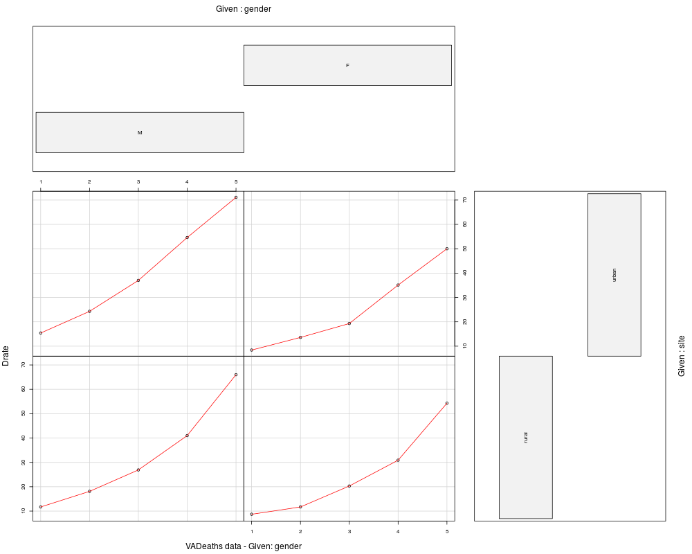
Death Rates in Virginia (1940)

Description

Death rates per 1000 in Virginia in 1940.

Usage

VADeaths

Format

A matrix with 5 rows and 4 columns.

Details

The death rates are measured per 1000 population per year. They are cross-classified by age group (rows) and population group (columns). The age groups are: 50–54, 55–59, 60–64, 65–69, 70–74 and the population groups are Rural/Male, Rural/Female, Urban/Male and Urban/Female.

This provides a rather nice 3-way analysis of variance example.

Source

Molyneaux, L., Gilliam, S. K., and Florant, L. C.(1947) Differences in Virginia death rates by color, sex, age, and rural or urban residence. American Sociological Review, 12, 525–535.

References

McNeil, D. R. (1977) Interactive Data Analysis. Wiley.

Examples

require(stats); require(graphics)
n <- length(dr <- c(VADeaths))
nam <- names(VADeaths)
d.VAD <- data.frame(
 Drate = dr,
 age = rep(ordered(rownames(VADeaths)), length.out = n),
 gender = gl(2, 5, n, labels = c("M", "F")),
 site =  gl(2, 10, labels = c("rural", "urban")))
coplot(Drate ~ as.numeric(age) | gender * site, data = d.VAD,
       panel = panel.smooth, xlab = "VADeaths data - Given: gender")
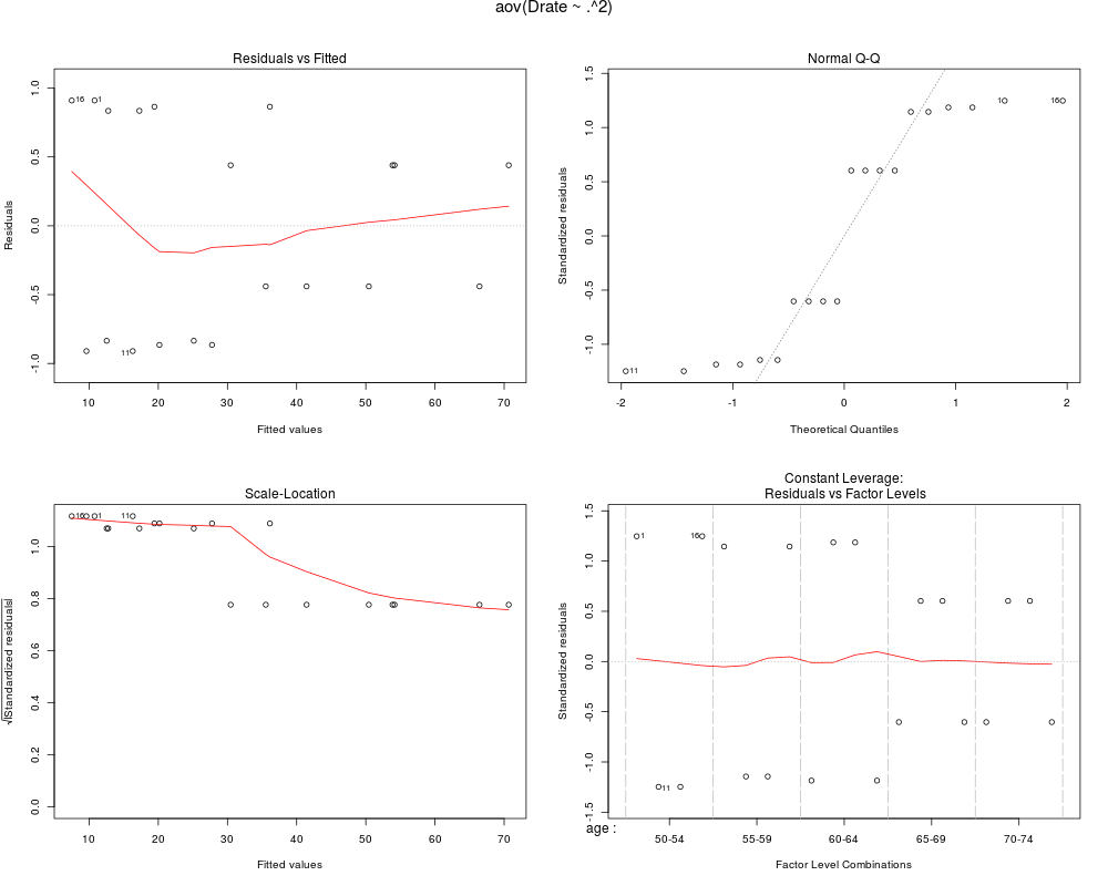
summary(aov.VAD <- aov(Drate ~ .^2, data = d.VAD))
opar <- par(mfrow = c(2, 2), oma = c(0, 0, 1.1, 0))
plot(aov.VAD)
par(opar)

Results

R version 3.3.1 (2016-06-21) -- "Bug in Your Hair"
Copyright (C) 2016 The R Foundation for Statistical Computing
Platform: x86_64-pc-linux-gnu (64-bit)

R is free software and comes with ABSOLUTELY NO WARRANTY.
You are welcome to redistribute it under certain conditions.
Type 'license()' or 'licence()' for distribution details.

R is a collaborative project with many contributors.
Type 'contributors()' for more information and
'citation()' on how to cite R or R packages in publications.

Type 'demo()' for some demos, 'help()' for on-line help, or
'help.start()' for an HTML browser interface to help.
Type 'q()' to quit R.

> library(datasets)
> png(filename="/home/ddbj/snapshot/RGM3/R_rel/result/datasets/VADeaths.Rd_%03d_medium.png", width=480, height=480)
> ### Name: VADeaths
> ### Title: Death Rates in Virginia (1940)
> ### Aliases: VADeaths
> ### Keywords: datasets
> 
> ### ** Examples
> 
> require(stats); require(graphics)
> n <- length(dr <- c(VADeaths))
> nam <- names(VADeaths)
> d.VAD <- data.frame(
+  Drate = dr,
+  age = rep(ordered(rownames(VADeaths)), length.out = n),
+  gender = gl(2, 5, n, labels = c("M", "F")),
+  site =  gl(2, 10, labels = c("rural", "urban")))
> coplot(Drate ~ as.numeric(age) | gender * site, data = d.VAD,
+        panel = panel.smooth, xlab = "VADeaths data - Given: gender")
> summary(aov.VAD <- aov(Drate ~ .^2, data = d.VAD))
            Df Sum Sq Mean Sq F value   Pr(>F)    
age          4   6288  1572.1 590.858 8.55e-06 ***
gender       1    648   647.5 243.361 9.86e-05 ***
site         1     77    76.8  28.876  0.00579 ** 
age:gender   4     86    21.6   8.100  0.03358 *  
age:site     4     43    10.6   3.996  0.10414    
gender:site  1     73    73.0  27.422  0.00636 ** 
Residuals    4     11     2.7                     
---
Signif. codes:  0 '***' 0.001 '**' 0.01 '*' 0.05 '.' 0.1 ' ' 1
> opar <- par(mfrow = c(2, 2), oma = c(0, 0, 1.1, 0))
> plot(aov.VAD)
> par(opar)
> 
> 
> 
> 
> 
> dev.off()
null device 
          1 
>