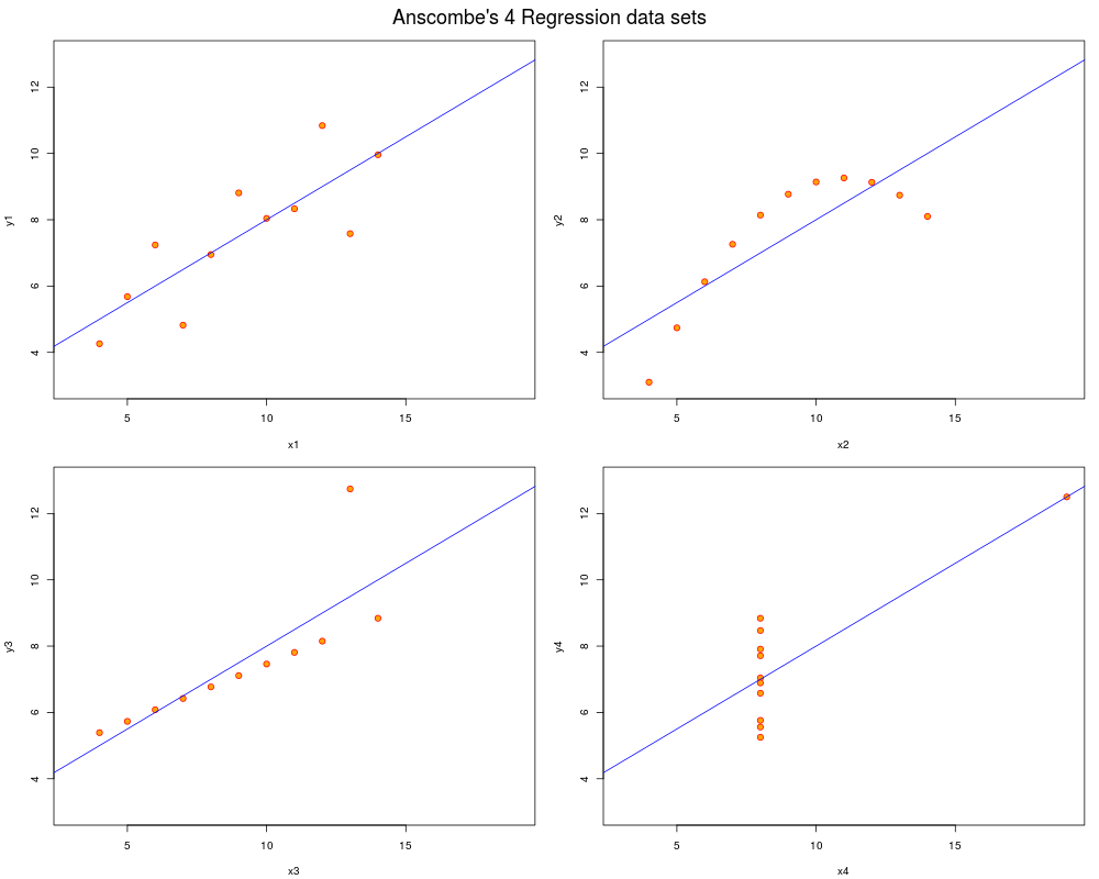
Anscombe's Quartet of ‘Identical’ Simple Linear Regressions

Description

Four x-y datasets which have the same traditional statistical properties (mean, variance, correlation, regression line, etc.), yet are quite different.

Usage

anscombe

Format

A data frame with 11 observations on 8 variables.

Source

Tufte, Edward R. (1989) The Visual Display of Quantitative Information, 13–14. Graphics Press.

References

Anscombe, Francis J. (1973) Graphs in statistical analysis. American Statistician, 27, 17–21.

Examples

require(stats); require(graphics)
summary(anscombe)

##-- now some "magic" to do the 4 regressions in a loop:
ff <- y ~ x
mods <- setNames(as.list(1:4), paste0("lm", 1:4))
for(i in 1:4) {
  ff[2:3] <- lapply(paste0(c("y","x"), i), as.name)
  ## or   ff[[2]] <- as.name(paste0("y", i))
  ##      ff[[3]] <- as.name(paste0("x", i))
  mods[[i]] <- lmi <- lm(ff, data = anscombe)
  print(anova(lmi))
}

## See how close they are (numerically!)
sapply(mods, coef)
lapply(mods, function(fm) coef(summary(fm)))

## Now, do what you should have done in the first place: PLOTS
op <- par(mfrow = c(2, 2), mar = 0.1+c(4,4,1,1), oma =  c(0, 0, 2, 0))
for(i in 1:4) {
  ff[2:3] <- lapply(paste0(c("y","x"), i), as.name)
  plot(ff, data = anscombe, col = "red", pch = 21, bg = "orange", cex = 1.2,
       xlim = c(3, 19), ylim = c(3, 13))
  abline(mods[[i]], col = "blue")
}
mtext("Anscombe's 4 Regression data sets", outer = TRUE, cex = 1.5)
par(op)

Results

R version 3.3.1 (2016-06-21) -- "Bug in Your Hair"
Copyright (C) 2016 The R Foundation for Statistical Computing
Platform: x86_64-pc-linux-gnu (64-bit)

R is free software and comes with ABSOLUTELY NO WARRANTY.
You are welcome to redistribute it under certain conditions.
Type 'license()' or 'licence()' for distribution details.

R is a collaborative project with many contributors.
Type 'contributors()' for more information and
'citation()' on how to cite R or R packages in publications.

Type 'demo()' for some demos, 'help()' for on-line help, or
'help.start()' for an HTML browser interface to help.
Type 'q()' to quit R.

> library(datasets)
> png(filename="/home/ddbj/snapshot/RGM3/R_rel/result/datasets/anscombe.Rd_%03d_medium.png", width=480, height=480)
> ### Name: anscombe
> ### Title: Anscombe's Quartet of 'Identical' Simple Linear Regressions
> ### Aliases: anscombe
> ### Keywords: datasets
> 
> ### ** Examples
> 
> require(stats); require(graphics)
> summary(anscombe)
       x1             x2             x3             x4           y1        
 Min.   : 4.0   Min.   : 4.0   Min.   : 4.0   Min.   : 8   Min.   : 4.260  
 1st Qu.: 6.5   1st Qu.: 6.5   1st Qu.: 6.5   1st Qu.: 8   1st Qu.: 6.315  
 Median : 9.0   Median : 9.0   Median : 9.0   Median : 8   Median : 7.580  
 Mean   : 9.0   Mean   : 9.0   Mean   : 9.0   Mean   : 9   Mean   : 7.501  
 3rd Qu.:11.5   3rd Qu.:11.5   3rd Qu.:11.5   3rd Qu.: 8   3rd Qu.: 8.570  
 Max.   :14.0   Max.   :14.0   Max.   :14.0   Max.   :19   Max.   :10.840  
       y2              y3              y4        
 Min.   :3.100   Min.   : 5.39   Min.   : 5.250  
 1st Qu.:6.695   1st Qu.: 6.25   1st Qu.: 6.170  
 Median :8.140   Median : 7.11   Median : 7.040  
 Mean   :7.501   Mean   : 7.50   Mean   : 7.501  
 3rd Qu.:8.950   3rd Qu.: 7.98   3rd Qu.: 8.190  
 Max.   :9.260   Max.   :12.74   Max.   :12.500  
> 
> ##-- now some "magic" to do the 4 regressions in a loop:
> ff <- y ~ x
> mods <- setNames(as.list(1:4), paste0("lm", 1:4))
> for(i in 1:4) {
+   ff[2:3] <- lapply(paste0(c("y","x"), i), as.name)
+   ## or   ff[[2]] <- as.name(paste0("y", i))
+   ##      ff[[3]] <- as.name(paste0("x", i))
+   mods[[i]] <- lmi <- lm(ff, data = anscombe)
+   print(anova(lmi))
+ }
Analysis of Variance Table

Response: y1
          Df Sum Sq Mean Sq F value  Pr(>F)   
x1         1 27.510 27.5100   17.99 0.00217 **
Residuals  9 13.763  1.5292                   
---
Signif. codes:  0 '***' 0.001 '**' 0.01 '*' 0.05 '.' 0.1 ' ' 1
Analysis of Variance Table

Response: y2
          Df Sum Sq Mean Sq F value   Pr(>F)   
x2         1 27.500 27.5000  17.966 0.002179 **
Residuals  9 13.776  1.5307                    
---
Signif. codes:  0 '***' 0.001 '**' 0.01 '*' 0.05 '.' 0.1 ' ' 1
Analysis of Variance Table

Response: y3
          Df Sum Sq Mean Sq F value   Pr(>F)   
x3         1 27.470 27.4700  17.972 0.002176 **
Residuals  9 13.756  1.5285                    
---
Signif. codes:  0 '***' 0.001 '**' 0.01 '*' 0.05 '.' 0.1 ' ' 1
Analysis of Variance Table

Response: y4
          Df Sum Sq Mean Sq F value   Pr(>F)   
x4         1 27.490 27.4900  18.003 0.002165 **
Residuals  9 13.742  1.5269                    
---
Signif. codes:  0 '***' 0.001 '**' 0.01 '*' 0.05 '.' 0.1 ' ' 1
> 
> ## See how close they are (numerically!)
> sapply(mods, coef)
                  lm1      lm2       lm3       lm4
(Intercept) 3.0000909 3.000909 3.0024545 3.0017273
x1          0.5000909 0.500000 0.4997273 0.4999091
> lapply(mods, function(fm) coef(summary(fm)))
$lm1
             Estimate Std. Error  t value    Pr(>|t|)
(Intercept) 3.0000909  1.1247468 2.667348 0.025734051
x1          0.5000909  0.1179055 4.241455 0.002169629

$lm2
            Estimate Std. Error  t value    Pr(>|t|)
(Intercept) 3.000909  1.1253024 2.666758 0.025758941
x2          0.500000  0.1179637 4.238590 0.002178816

$lm3
             Estimate Std. Error  t value    Pr(>|t|)
(Intercept) 3.0024545  1.1244812 2.670080 0.025619109
x3          0.4997273  0.1178777 4.239372 0.002176305

$lm4
             Estimate Std. Error  t value    Pr(>|t|)
(Intercept) 3.0017273  1.1239211 2.670763 0.025590425
x4          0.4999091  0.1178189 4.243028 0.002164602

> 
> ## Now, do what you should have done in the first place: PLOTS
> op <- par(mfrow = c(2, 2), mar = 0.1+c(4,4,1,1), oma =  c(0, 0, 2, 0))
> for(i in 1:4) {
+   ff[2:3] <- lapply(paste0(c("y","x"), i), as.name)
+   plot(ff, data = anscombe, col = "red", pch = 21, bg = "orange", cex = 1.2,
+        xlim = c(3, 19), ylim = c(3, 13))
+   abline(mods[[i]], col = "blue")
+ }
> mtext("Anscombe's 4 Regression data sets", outer = TRUE, cex = 1.5)
> par(op)
> 
> 
> 
> 
> 
> dev.off()
null device 
          1 
>