Smoking, Alcohol and (O)esophageal Cancer

Description

Data from a case-control study of (o)esophageal cancer in Ille-et-Vilaine, France.

Usage

esoph

Format

A data frame with records for 88 age/alcohol/tobacco combinations.

Author(s)

Thomas Lumley

Source

Breslow, N. E. and Day, N. E. (1980) Statistical Methods in Cancer Research. Volume 1: The Analysis of Case-Control Studies. IARC Lyon / Oxford University Press.

Examples

require(stats)
require(graphics) # for mosaicplot
summary(esoph)
## effects of alcohol, tobacco and interaction, age-adjusted
model1 <- glm(cbind(ncases, ncontrols) ~ agegp + tobgp * alcgp,
              data = esoph, family = binomial())
anova(model1)
## Try a linear effect of alcohol and tobacco
model2 <- glm(cbind(ncases, ncontrols) ~ agegp + unclass(tobgp)
                                         + unclass(alcgp),
              data = esoph, family = binomial())
summary(model2)
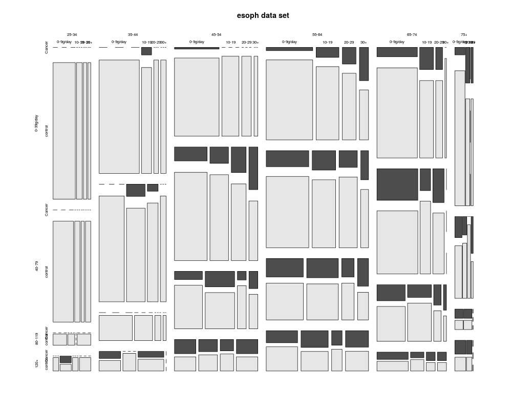
## Re-arrange data for a mosaic plot
ttt <- table(esoph$agegp, esoph$alcgp, esoph$tobgp)
o <- with(esoph, order(tobgp, alcgp, agegp))
ttt[ttt == 1] <- esoph$ncases[o]
tt1 <- table(esoph$agegp, esoph$alcgp, esoph$tobgp)
tt1[tt1 == 1] <- esoph$ncontrols[o]
tt <- array(c(ttt, tt1), c(dim(ttt),2),
            c(dimnames(ttt), list(c("Cancer", "control"))))
mosaicplot(tt, main = "esoph data set", color = TRUE)

Results

R version 3.3.1 (2016-06-21) -- "Bug in Your Hair"
Copyright (C) 2016 The R Foundation for Statistical Computing
Platform: x86_64-pc-linux-gnu (64-bit)

R is free software and comes with ABSOLUTELY NO WARRANTY.
You are welcome to redistribute it under certain conditions.
Type 'license()' or 'licence()' for distribution details.

R is a collaborative project with many contributors.
Type 'contributors()' for more information and
'citation()' on how to cite R or R packages in publications.

Type 'demo()' for some demos, 'help()' for on-line help, or
'help.start()' for an HTML browser interface to help.
Type 'q()' to quit R.

> library(datasets)
> png(filename="/home/ddbj/snapshot/RGM3/R_rel/result/datasets/esoph.Rd_%03d_medium.png", width=480, height=480)
> ### Name: esoph
> ### Title: Smoking, Alcohol and (O)esophageal Cancer
> ### Aliases: esoph
> ### Keywords: datasets
> 
> ### ** Examples
> 
> require(stats)
> require(graphics) # for mosaicplot
> summary(esoph)
   agegp          alcgp         tobgp        ncases         ncontrols    
 25-34:15   0-39g/day:23   0-9g/day:24   Min.   : 0.000   Min.   : 1.00  
 35-44:15   40-79    :23   10-19   :24   1st Qu.: 0.000   1st Qu.: 3.00  
 45-54:16   80-119   :21   20-29   :20   Median : 1.000   Median : 6.00  
 55-64:16   120+     :21   30+     :20   Mean   : 2.273   Mean   :11.08  
 65-74:15                                3rd Qu.: 4.000   3rd Qu.:14.00  
 75+  :11                                Max.   :17.000   Max.   :60.00  
> ## effects of alcohol, tobacco and interaction, age-adjusted
> model1 <- glm(cbind(ncases, ncontrols) ~ agegp + tobgp * alcgp,
+               data = esoph, family = binomial())
> anova(model1)
Analysis of Deviance Table

Model: binomial, link: logit

Response: cbind(ncases, ncontrols)

Terms added sequentially (first to last)


            Df Deviance Resid. Df Resid. Dev
NULL                           87    227.241
agegp        5   88.128        82    139.112
tobgp        3   19.085        79    120.028
alcgp        3   66.054        76     53.973
tobgp:alcgp  9    6.489        67     47.484
> ## Try a linear effect of alcohol and tobacco
> model2 <- glm(cbind(ncases, ncontrols) ~ agegp + unclass(tobgp)
+                                          + unclass(alcgp),
+               data = esoph, family = binomial())
> summary(model2)

Call:
glm(formula = cbind(ncases, ncontrols) ~ agegp + unclass(tobgp) + 
    unclass(alcgp), family = binomial(), data = esoph)

Deviance Residuals: 
    Min       1Q   Median       3Q      Max  
-1.7628  -0.6426  -0.2709   0.3043   2.0421  

Coefficients:
               Estimate Std. Error z value Pr(>|z|)    
(Intercept)    -4.01097    0.31224 -12.846  < 2e-16 ***
agegp.L         2.96113    0.65092   4.549 5.39e-06 ***
agegp.Q        -1.33735    0.58918  -2.270  0.02322 *  
agegp.C         0.15292    0.44792   0.341  0.73281    
agegp^4         0.06668    0.30776   0.217  0.82848    
agegp^5        -0.20288    0.19523  -1.039  0.29872    
unclass(tobgp)  0.26162    0.08198   3.191  0.00142 ** 
unclass(alcgp)  0.65308    0.08452   7.727 1.10e-14 ***
---
Signif. codes:  0 '***' 0.001 '**' 0.01 '*' 0.05 '.' 0.1 ' ' 1

(Dispersion parameter for binomial family taken to be 1)

    Null deviance: 227.241  on 87  degrees of freedom
Residual deviance:  59.277  on 80  degrees of freedom
AIC: 222.76

Number of Fisher Scoring iterations: 6

> ## Re-arrange data for a mosaic plot
> ttt <- table(esoph$agegp, esoph$alcgp, esoph$tobgp)
> o <- with(esoph, order(tobgp, alcgp, agegp))
> ttt[ttt == 1] <- esoph$ncases[o]
> tt1 <- table(esoph$agegp, esoph$alcgp, esoph$tobgp)
> tt1[tt1 == 1] <- esoph$ncontrols[o]
> tt <- array(c(ttt, tt1), c(dim(ttt),2),
+             c(dimnames(ttt), list(c("Cancer", "control"))))
> mosaicplot(tt, main = "esoph data set", color = TRUE)
> 
> 
> 
> 
> 
> dev.off()
null device 
          1 
>