Longley's Economic Regression Data

Description

A macroeconomic data set which provides a well-known example for a highly collinear regression.

Usage

longley

Format

A data frame with 7 economical variables, observed yearly from 1947 to 1962 (n=16).

GNP.deflator

GNP implicit price deflator (1954=100)

GNP

Gross National Product.

Unemployed

number of unemployed.

Armed.Forces

number of people in the armed forces.

Population

‘noninstitutionalized’ population ≥ 14 years of age.

Year

the year (time).

Employed

number of people employed.

The regression lm(Employed ~ .) is known to be highly collinear.

Source

J. W. Longley (1967) An appraisal of least-squares programs from the point of view of the user. Journal of the American Statistical Association 62, 819–841.

References

Becker, R. A., Chambers, J. M. and Wilks, A. R. (1988) The New S Language. Wadsworth & Brooks/Cole.

Examples

require(stats); require(graphics)
## give the data set in the form it is used in S-PLUS:
longley.x <- data.matrix(longley[, 1:6])
longley.y <- longley[, "Employed"]
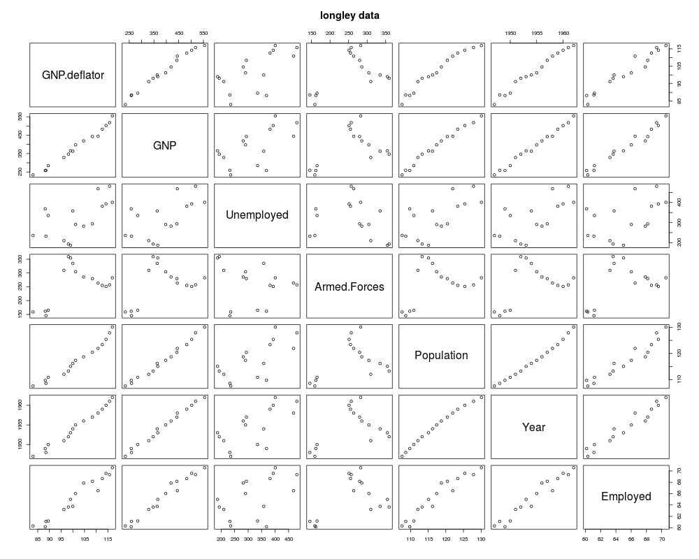
pairs(longley, main = "longley data")
summary(fm1 <- lm(Employed ~ ., data = longley))
opar <- par(mfrow = c(2, 2), oma = c(0, 0, 1.1, 0),
            mar = c(4.1, 4.1, 2.1, 1.1))
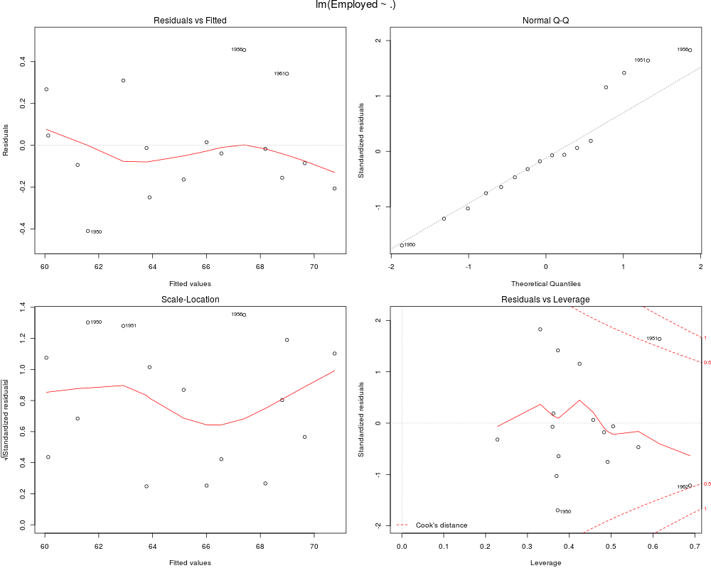
plot(fm1)
par(opar)

Results

R version 3.3.1 (2016-06-21) -- "Bug in Your Hair"
Copyright (C) 2016 The R Foundation for Statistical Computing
Platform: x86_64-pc-linux-gnu (64-bit)

R is free software and comes with ABSOLUTELY NO WARRANTY.
You are welcome to redistribute it under certain conditions.
Type 'license()' or 'licence()' for distribution details.

R is a collaborative project with many contributors.
Type 'contributors()' for more information and
'citation()' on how to cite R or R packages in publications.

Type 'demo()' for some demos, 'help()' for on-line help, or
'help.start()' for an HTML browser interface to help.
Type 'q()' to quit R.

> library(datasets)
> png(filename="/home/ddbj/snapshot/RGM3/R_rel/result/datasets/longley.Rd_%03d_medium.png", width=480, height=480)
> ### Name: longley
> ### Title: Longley's Economic Regression Data
> ### Aliases: longley
> ### Keywords: datasets
> 
> ### ** Examples
> 
> require(stats); require(graphics)
> ## give the data set in the form it is used in S-PLUS:
> longley.x <- data.matrix(longley[, 1:6])
> longley.y <- longley[, "Employed"]
> pairs(longley, main = "longley data")
> summary(fm1 <- lm(Employed ~ ., data = longley))

Call:
lm(formula = Employed ~ ., data = longley)

Residuals:
     Min       1Q   Median       3Q      Max 
-0.41011 -0.15767 -0.02816  0.10155  0.45539 

Coefficients:
               Estimate Std. Error t value Pr(>|t|)    
(Intercept)  -3.482e+03  8.904e+02  -3.911 0.003560 ** 
GNP.deflator  1.506e-02  8.492e-02   0.177 0.863141    
GNP          -3.582e-02  3.349e-02  -1.070 0.312681    
Unemployed   -2.020e-02  4.884e-03  -4.136 0.002535 ** 
Armed.Forces -1.033e-02  2.143e-03  -4.822 0.000944 ***
Population   -5.110e-02  2.261e-01  -0.226 0.826212    
Year          1.829e+00  4.555e-01   4.016 0.003037 ** 
---
Signif. codes:  0 '***' 0.001 '**' 0.01 '*' 0.05 '.' 0.1 ' ' 1

Residual standard error: 0.3049 on 9 degrees of freedom
Multiple R-squared:  0.9955,	Adjusted R-squared:  0.9925 
F-statistic: 330.3 on 6 and 9 DF,  p-value: 4.984e-10

> opar <- par(mfrow = c(2, 2), oma = c(0, 0, 1.1, 0),
+             mar = c(4.1, 4.1, 2.1, 1.1))
> plot(fm1)
> par(opar)
> 
> 
> 
> 
> 
> dev.off()
null device 
          1 
>