Supported by Dr. Osamu Ogasawara and  . . |
|
Last data update: 2014.03.03 |
Generic autoplot functionDescription
Usage
## S4 method for signature 'GRanges'
autoplot(object, ..., chr, xlab, ylab, main, truncate.gaps = FALSE,
                 truncate.fun = NULL, ratio = 0.0025, space.skip = 0.1,
                 legend = TRUE, geom = NULL, stat = NULL,
                 chr.weight = NULL,
                 coord = c("default", "genome", "truncate_gaps"),
                 layout = c("linear", "karyogram", "circle"))


## S4 method for signature 'GRangesList'
autoplot(object, ..., xlab, ylab, main, indName = "grl_name",
                 geom = NULL, stat = NULL, coverage.col = "gray50",
                 coverage.fill = coverage.col, group.selfish = FALSE)


## S4 method for signature 'IRanges'
autoplot(object, ..., xlab, ylab, main)

## S4 method for signature 'Seqinfo'
autoplot(object, ideogram = FALSE, ... )

## S4 method for signature 'GAlignments'
autoplot(object, ..., xlab, ylab, main, which,
      geom = NULL, stat = NULL)

## S4 method for signature 'BamFile'
autoplot(object, ..., which, xlab, ylab, main,
                 bsgenome, geom = "line", stat = "coverage", method = c("raw",
                 "estimate"), coord = c("linear", "genome"),
                 resize.extra = 10, space.skip = 0.1, show.coverage =
                 TRUE)


## S4 method for signature 'character'
autoplot(object, ..., xlab, ylab, main, which)

## S4 method for signature 'TxDbOREnsDb'
autoplot(object, which, ..., xlab, ylab, main, truncate.gaps =
                 FALSE, truncate.fun = NULL, ratio = 0.0025,
                 mode = c("full", "reduce"),geom =
                 c("alignment"), stat = c("identity", "reduce"),
                 names.expr = "tx_name", label = TRUE)


## S4 method for signature 'BSgenome'
autoplot(object, which, ...,
                    xlab, ylab, main, geom = NULL)


## S4 method for signature 'Rle'
autoplot(object, ..., xlab, ylab, main, binwidth, nbin = 30,
          geom = NULL, stat = c("bin", "identity", "slice"),
          type = c("viewSums", "viewMins", "viewMaxs", "viewMeans"))

## S4 method for signature 'RleList'
autoplot(object, ..., xlab, ylab, main, nbin = 30, binwidth,
         facetByRow = TRUE, stat = c("bin", "identity", "slice"),
         geom = NULL, type = c("viewSums", "viewMins", "viewMaxs", "viewMeans"))

## S4 method for signature 'matrix'
autoplot(object, ..., xlab, ylab, main,
              geom = c("tile", "raster"), axis.text.angle = NULL,
              hjust = 0.5, na.value = NULL,
              rownames.label = TRUE, colnames.label = TRUE,
              axis.text.x = TRUE, axis.text.y = TRUE)


## S4 method for signature 'ExpressionSet'
autoplot(object, ..., type = c("heatmap", "none",
                 "scatterplot.matrix", "pcp", "MA", "boxplot",
                 "mean-sd"), test.method =
                 "t", rotate = FALSE, pheno.plot = FALSE, main_to_pheno
                 = 4.5, padding = 0.2)


## S4 method for signature 'RangedSummarizedExperiment'
autoplot(object, ..., type = c("heatmap", "link", "pcp", "boxplot", "scatterplot.matrix"), pheno.plot = FALSE,
                 main_to_pheno = 4.5, padding = 0.2, assay.id = 1)


## S4 method for signature 'VCF'
autoplot(object, ...,
              xlab, ylab, main,
              assay.id,
              type = c("default", "geno", "info", "fixed"),
              full.string = FALSE,
              ref.show = TRUE,
              genome.axis = TRUE,
              transpose = TRUE)

## S4 method for signature 'OrganismDb'
autoplot(object, which, ...,
                   xlab, ylab, main,
                   truncate.gaps = FALSE,
                   truncate.fun = NULL,
                   ratio = 0.0025,
                   geom = c("alignment"),
                   stat = c("identity", "reduce"),
                   columns = c("TXNAME", "SYMBOL", "TXID", "GENEID"),
                   names.expr = "SYMBOL",
                   label = TRUE,
                   label.color = "gray40")

## S4 method for signature 'VRanges'
autoplot(object, ...,which = NULL,
                             arrow = TRUE, indel.col = "gray30",
                             geom = NULL,
                             xlab, ylab, main)

## S4 method for signature 'TabixFile'
autoplot(object, which, ...)
Arguments
ValueA Introduction
GeometryWe have developed new This package is designed for only biological data, especially genomic
data if users want to explore the data in a more flexible way, you
could simply coerce the Some objects share the same geom so we introduce all the geom together in this section
FacetingFaceting in ggbio package is a little differnt from ggplot2 in several ways
Author(s)Tengfei Yin Examples
library(ggbio)
set.seed(1)
N <- 1000
library(GenomicRanges)
gr <- GRanges(seqnames =
sample(c("chr1", "chr2", "chr3"),
size = N, replace = TRUE),
IRanges(
start = sample(1:300, size = N, replace = TRUE),
width = sample(70:75, size = N,replace = TRUE)),
strand = sample(c("+", "-", "*"), size = N,
replace = TRUE),
value = rnorm(N, 10, 3), score = rnorm(N, 100, 30),
sample = sample(c("Normal", "Tumor"),
size = N, replace = TRUE),
pair = sample(letters, size = N,
replace = TRUE))
idx <- sample(1:length(gr), size = 50)
###################################################
### code chunk number 3: default
###################################################
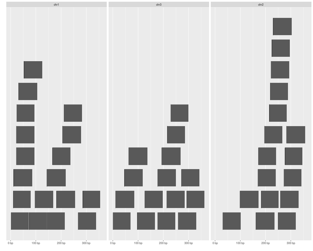
autoplot(gr[idx])
###################################################
### code chunk number 4: bar-default-pre
###################################################
set.seed(123)
gr.b <- GRanges(seqnames = "chr1", IRanges(start = seq(1, 100, by = 10),
width = sample(4:9, size = 10, replace = TRUE)),
score = rnorm(10, 10, 3), value = runif(10, 1, 100))
gr.b2 <- GRanges(seqnames = "chr2", IRanges(start = seq(1, 100, by = 10),
width = sample(4:9, size = 10, replace = TRUE)),
score = rnorm(10, 10, 3), value = runif(10, 1, 100))
gr.b <- c(gr.b, gr.b2)
head(gr.b)
###################################################
### code chunk number 5: bar-default
###################################################
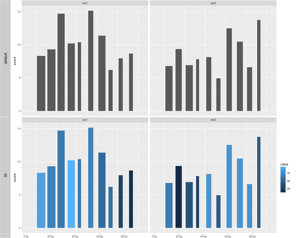
p1 <- autoplot(gr.b, geom = "bar")
## use value to fill the bar
p2 <- autoplot(gr.b, geom = "bar", aes(fill = value))
tracks(default = p1, fill = p2)
###################################################
### code chunk number 6: autoplot.Rnw:236-237
###################################################
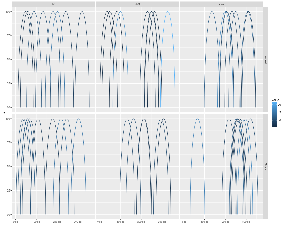
autoplot(gr[idx], geom = "arch", aes(color = value), facets = sample ~ seqnames)
###################################################
### code chunk number 7: gr-group
###################################################
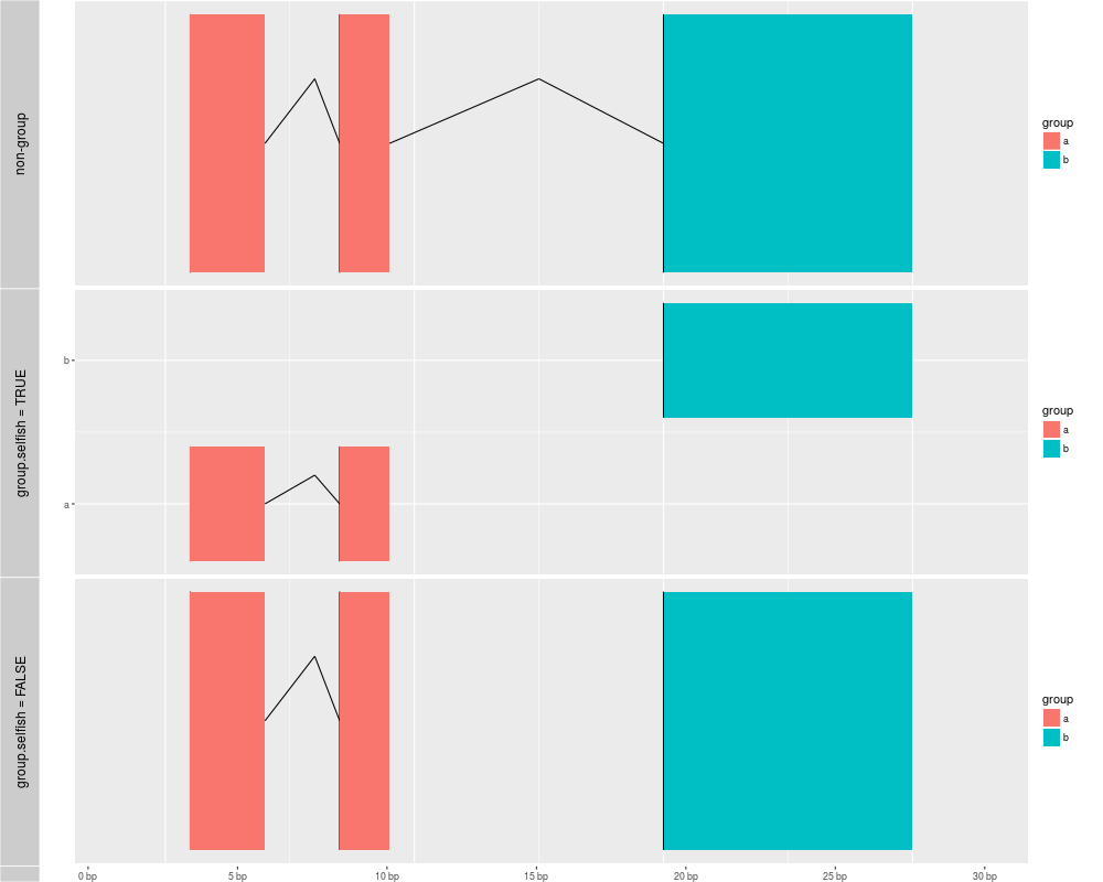
gra <- GRanges("chr1", IRanges(c(1,7,20), end = c(4,9,30)), group = c("a", "a", "b"))
## if you desn't specify group, then group based on stepping levels, and gaps are computed without
## considering extra group method
p1 <- autoplot(gra, aes(fill = group), geom = "alignment")
## when use group method, gaps only computed for grouped intervals.
## default is group.selfish = TRUE, each group keep one row.
## in this way, group labels could be shown as y axis.
p2 <- autoplot(gra, aes(fill = group, group = group), geom = "alignment")
## group.selfish = FALSE, save space
p3 <- autoplot(gra, aes(fill = group, group = group), geom = "alignment", group.selfish = FALSE)
tracks('non-group' = p1,'group.selfish = TRUE' = p2 , 'group.selfish = FALSE' = p3)
###################################################
### code chunk number 8: gr-facet-strand
###################################################
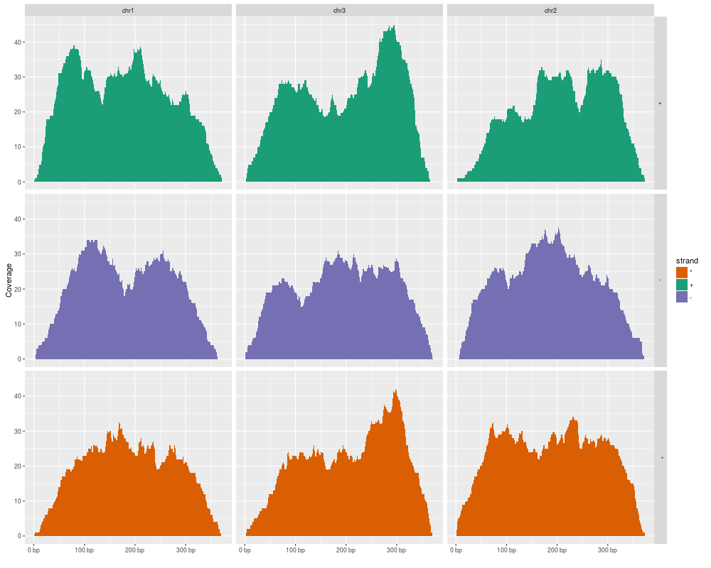
autoplot(gr, stat = "coverage", geom = "area",
facets = strand ~ seqnames, aes(fill = strand))
###################################################
### code chunk number 9: gr-autoplot-circle
###################################################
autoplot(gr[idx], layout = 'circle')
###################################################
### code chunk number 10: gr-circle
###################################################
seqlengths(gr) <- c(400, 500, 700)
values(gr)$to.gr <- gr[sample(1:length(gr), size = length(gr))]
idx <- sample(1:length(gr), size = 50)
gr <- gr[idx]
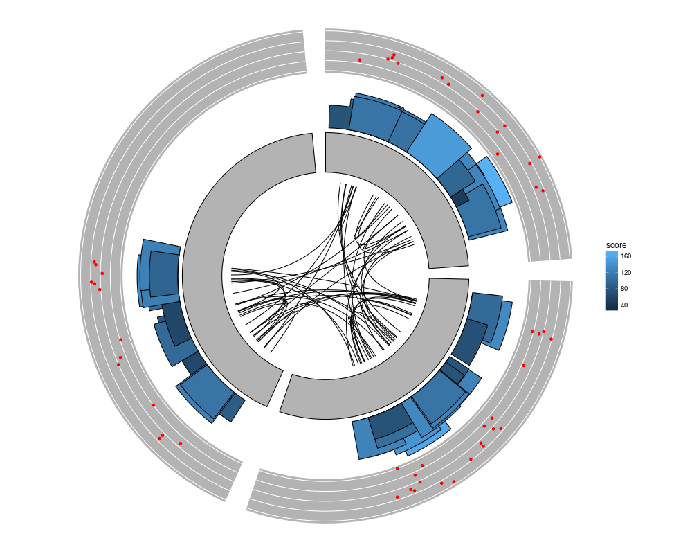
ggplot() + layout_circle(gr, geom = "ideo", fill = "gray70", radius = 7, trackWidth = 3) +
layout_circle(gr, geom = "bar", radius = 10, trackWidth = 4,
aes(fill = score, y = score)) +
layout_circle(gr, geom = "point", color = "red", radius = 14,
trackWidth = 3, grid = TRUE, aes(y = score)) +
layout_circle(gr, geom = "link", linked.to = "to.gr", radius = 6, trackWidth = 1)
###################################################
### code chunk number 11: seqinfo-src
###################################################
data(hg19Ideogram, package = "biovizBase")
sq <- seqinfo(hg19Ideogram)
sq
###################################################
### code chunk number 12: seqinfo
###################################################
autoplot(sq[paste0("chr", c(1:22, "X"))])
###################################################
### code chunk number 13: ir-load
###################################################
set.seed(1)
N <- 100
ir <- IRanges(start = sample(1:300, size = N, replace = TRUE),
width = sample(70:75, size = N,replace = TRUE))
## add meta data
df <- DataFrame(value = rnorm(N, 10, 3), score = rnorm(N, 100, 30),
sample = sample(c("Normal", "Tumor"),
size = N, replace = TRUE),
pair = sample(letters, size = N,
replace = TRUE))
values(ir) <- df
ir
###################################################
### code chunk number 14: ir-exp
###################################################
p1 <- autoplot(ir)
p2 <- autoplot(ir, aes(fill = pair)) + theme(legend.position = "none")
p3 <- autoplot(ir, stat = "coverage", geom = "line", facets = sample ~. )
p4 <- autoplot(ir, stat = "reduce")
tracks(p1, p2, p3, p4)
###################################################
### code chunk number 15: grl-simul
###################################################
set.seed(1)
N <- 100
## ======================================================================
## simmulated GRanges
## ======================================================================
gr <- GRanges(seqnames =
sample(c("chr1", "chr2", "chr3"),
size = N, replace = TRUE),
IRanges(
start = sample(1:300, size = N, replace = TRUE),
width = sample(30:40, size = N,replace = TRUE)),
strand = sample(c("+", "-", "*"), size = N,
replace = TRUE),
value = rnorm(N, 10, 3), score = rnorm(N, 100, 30),
sample = sample(c("Normal", "Tumor"),
size = N, replace = TRUE),
pair = sample(letters, size = N,
replace = TRUE))
grl <- split(gr, values(gr)$pair)
###################################################
### code chunk number 16: grl-exp
###################################################
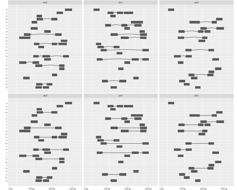
## default gap.geom is 'chevron'
p1 <- autoplot(grl, group.selfish = TRUE)
p2 <- autoplot(grl, group.selfish = TRUE, main.geom = "arrowrect", gap.geom = "segment")
tracks(p1, p2)
###################################################
### code chunk number 17: grl-name
###################################################
autoplot(grl, aes(fill = ..grl_name..))
## equal to
## autoplot(grl, aes(fill = grl_name))
###################################################
### code chunk number 18: rle-simul
###################################################
library(IRanges)
set.seed(1)
lambda <- c(rep(0.001, 4500), seq(0.001, 10, length = 500),
seq(10, 0.001, length = 500))
## @knitr create
xVector <- rpois(1e4, lambda)
xRle <- Rle(xVector)
xRle
###################################################
### code chunk number 19: rle-bin
###################################################
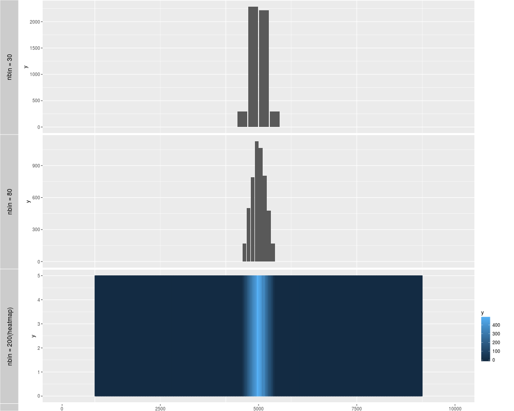
p1 <- autoplot(xRle)
p2 <- autoplot(xRle, nbin = 80)
p3 <- autoplot(xRle, geom = "heatmap", nbin = 200)
tracks('nbin = 30' = p1, "nbin = 80" = p2, "nbin = 200(heatmap)" = p3)
###################################################
### code chunk number 20: rle-id
###################################################
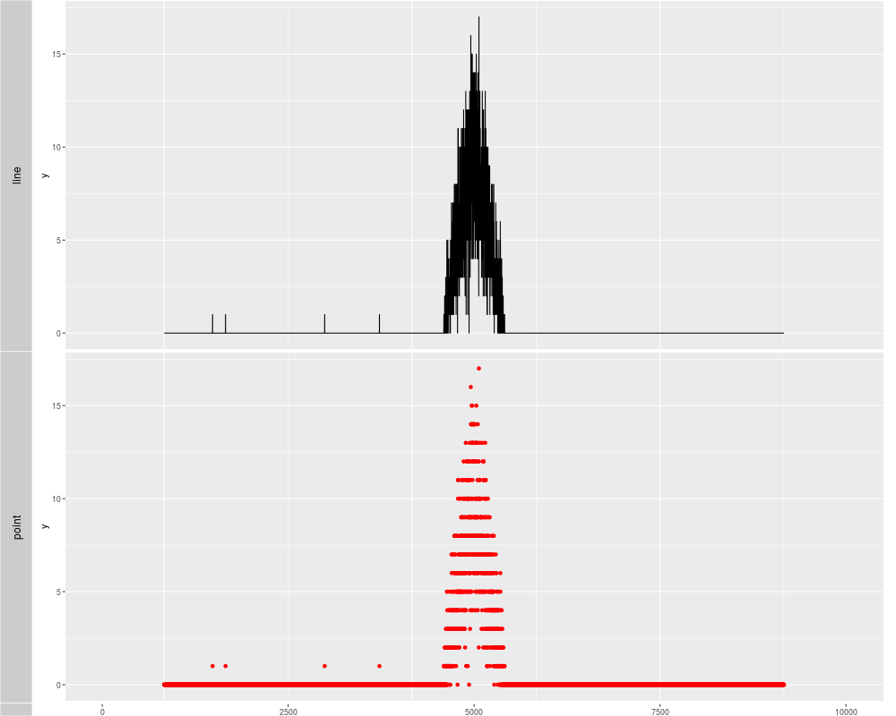
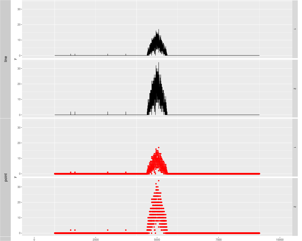
p1 <- autoplot(xRle, stat = "identity")
p2 <- autoplot(xRle, stat = "identity", geom = "point", color = "red")
tracks('line' = p1, "point" = p2)
###################################################
### code chunk number 21: rle-slice
###################################################
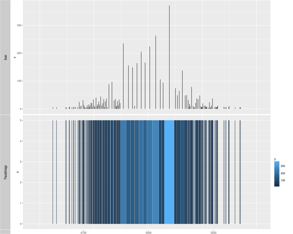
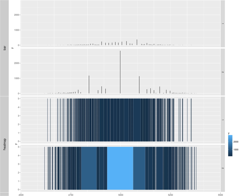
p1 <- autoplot(xRle, type = "viewMaxs", stat = "slice", lower = 5)
p2 <- autoplot(xRle, type = "viewMaxs", stat = "slice", lower = 5, geom = "heatmap")
tracks('bar' = p1, "heatmap" = p2)
###################################################
### code chunk number 22: rlel-simul
###################################################
xRleList <- RleList(xRle, 2L * xRle)
xRleList
###################################################
### code chunk number 23: rlel-bin
###################################################
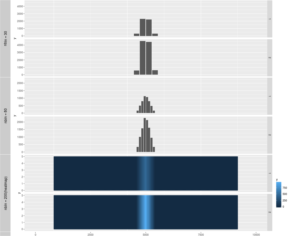
p1 <- autoplot(xRleList)
p2 <- autoplot(xRleList, nbin = 80)
p3 <- autoplot(xRleList, geom = "heatmap", nbin = 200)
tracks('nbin = 30' = p1, "nbin = 80" = p2, "nbin = 200(heatmap)" = p3)
###################################################
### code chunk number 24: rlel-id
###################################################
p1 <- autoplot(xRleList, stat = "identity")
p2 <- autoplot(xRleList, stat = "identity", geom = "point", color = "red")
tracks('line' = p1, "point" = p2)
###################################################
### code chunk number 25: rlel-slice
###################################################
p1 <- autoplot(xRleList, type = "viewMaxs", stat = "slice", lower = 5)
p2 <- autoplot(xRleList, type = "viewMaxs", stat = "slice", lower = 5, geom = "heatmap")
tracks('bar' = p1, "heatmap" = p2)
###################################################
### code chunk number 26: txdb
###################################################
library(TxDb.Hsapiens.UCSC.hg19.knownGene)
data(genesymbol, package = "biovizBase")
txdb <- TxDb.Hsapiens.UCSC.hg19.knownGene
###################################################
### code chunk number 27: txdb-visual
###################################################
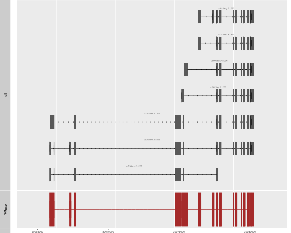
p1 <- autoplot(txdb, which = genesymbol["ALDOA"], names.expr = "tx_name:::gene_id")
p2 <- autoplot(txdb, which = genesymbol["ALDOA"], stat = "reduce", color = "brown",
fill = "brown")
tracks(full = p1, reduce = p2, heights = c(5, 1)) + ylab("")
###################################################
### EnsDb
###################################################
## Fetching gene models from an EnsDb object.
library(EnsDb.Hsapiens.v75)
ensdb <- EnsDb.Hsapiens.v75
## We use a GenenameFilter to specifically retrieve all transcripts for that gene.
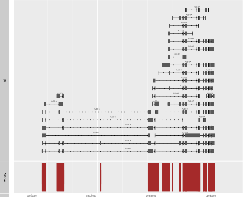
p1 <- autoplot(ensdb, which=GenenameFilter("ALDOA"), names.expr="gene_name")
p2 <- autoplot(ensdb, which=GenenameFilter("ALDOA"), stat="reduce", color="brown",
fill="brown")
tracks(full = p1, reduce = p2, heights = c(5, 1)) + ylab("")
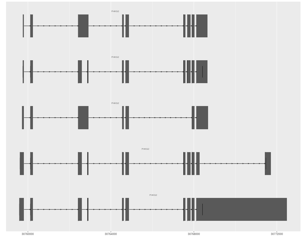
## Alternatively, we can specify a GRangesFilter and display all genes
## that are (partially) overlapping with that genomic region:
gr <- GRanges(seqnames=16, IRanges(30768000, 30770000), strand="+")
autoplot(ensdb, GRangesFilter(gr, "overlapping"), names.expr="gene_name")
## Just submitting the GRanges object also works.
autoplot(ensdb, gr, names.expr="gene_name")
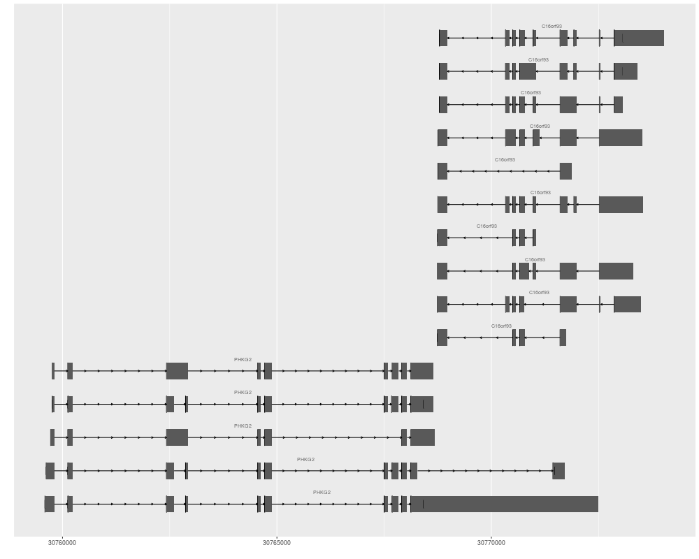
## Or genes encoded on both strands.
gr <- GRanges(seqnames=16, IRanges(30768000, 30770000), strand="*")
autoplot(ensdb, GRangesFilter(gr, "overlapping"), names.expr="gene_name")
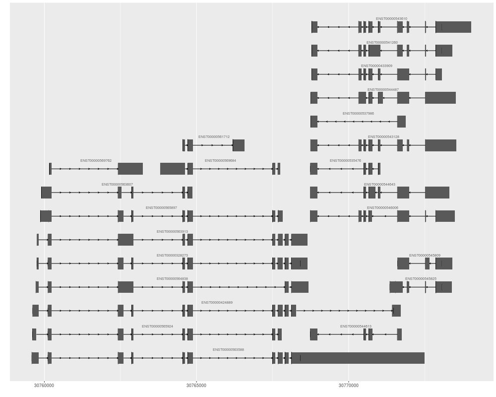
## Also, we can spefify directly the gene ids and plot all transcripts of these
## genes (not only those overlapping with the region)
autoplot(ensdb, GeneidFilter(c("ENSG00000196118", "ENSG00000156873")))
###################################################
### code chunk number 28: ga-load
###################################################
library(GenomicAlignments)
data("genesymbol", package = "biovizBase")
bamfile <- system.file("extdata", "SRR027894subRBM17.bam",
package="biovizBase")
which <- keepStandardChromosomes(genesymbol["RBM17"])
## need to set use.names = TRUE
ga <- readGAlignments(bamfile,
param = ScanBamParam(which = which),
use.names = TRUE)
###################################################
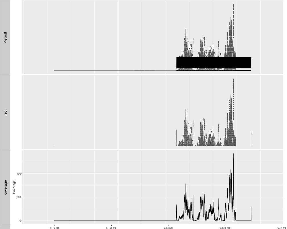
### code chunk number 29: ga-exp
###################################################
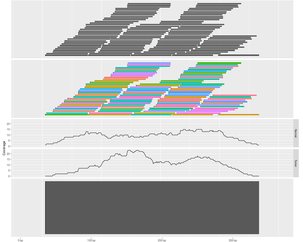
p1 <- autoplot(ga)
p2 <- autoplot(ga, geom = "rect")
p3 <- autoplot(ga, geom = "line", stat = "coverage")
tracks(default = p1, rect = p2, coverage = p3)
###################################################
### code chunk number 30: bf-load (eval = FALSE)
###################################################
## library(Rsamtools)
## bamfile <- "./wgEncodeCaltechRnaSeqK562R1x75dAlignsRep1V2.bam"
## bf <- BamFile(bamfile)
###################################################
### code chunk number 31: bf-est-cov (eval = FALSE)
###################################################
## autoplot(bamfile)
## autoplot(bamfile, which = c("chr1", "chr2"))
## autoplot(bf)
## autoplot(bf, which = c("chr1", "chr2"))
##
## data(genesymbol, package = "biovizBase")
## autoplot(bamfile, method = "raw", which = genesymbol["ALDOA"])
##
## library(BSgenome.Hsapiens.UCSC.hg19)
## autoplot(bf, stat = "mismatch", which = genesymbol["ALDOA"], bsgenome = Hsapiens)
###################################################
### code chunk number 32: char-bam (eval = FALSE)
###################################################
## bamfile <- "./wgEncodeCaltechRnaSeqK562R1x75dAlignsRep1V2.bam"
## autoplot(bamfile)
###################################################
### code chunk number 33: char-gr
###################################################
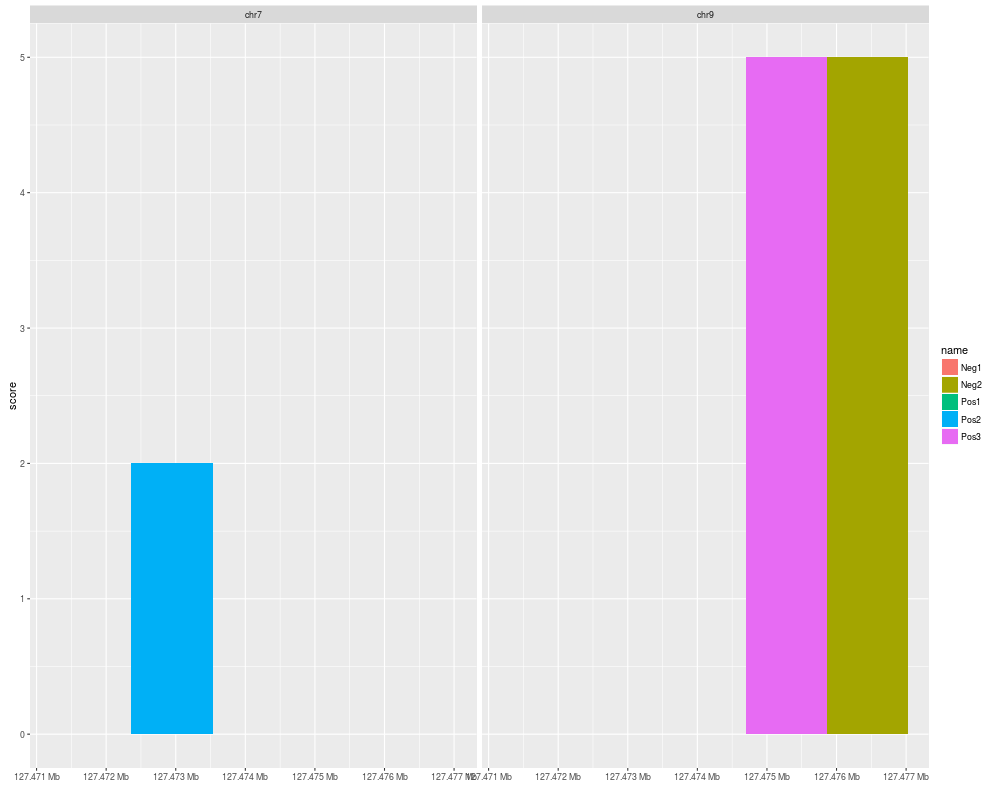
library(rtracklayer)
test_path <- system.file("tests", package = "rtracklayer")
test_bed <- file.path(test_path, "test.bed")
autoplot(test_bed, aes(fill = name))
###################################################
### matrix
###################################################
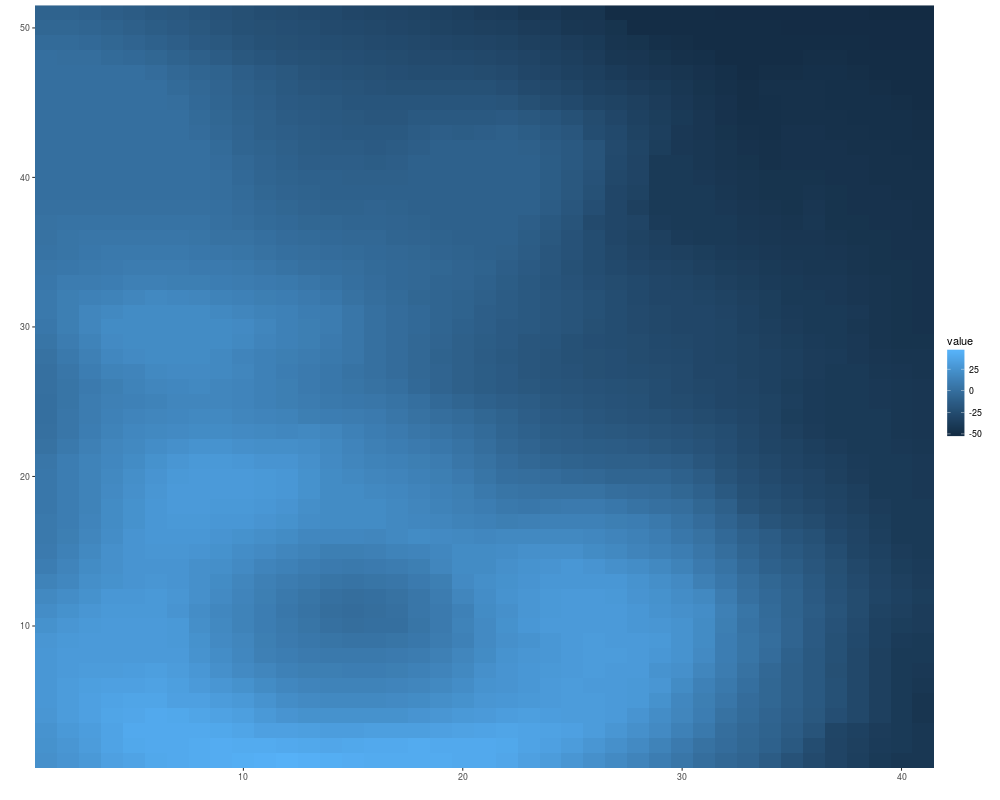
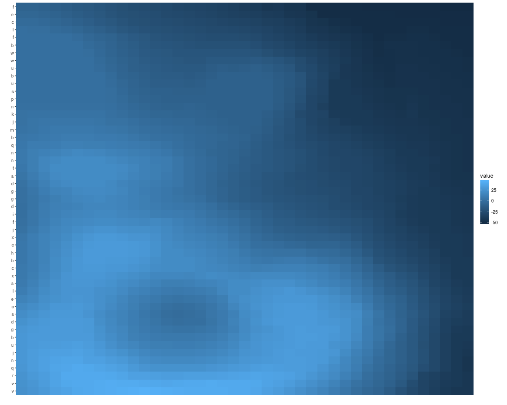
volcano <- volcano[20:70, 20:60] - 150
autoplot(volcano)
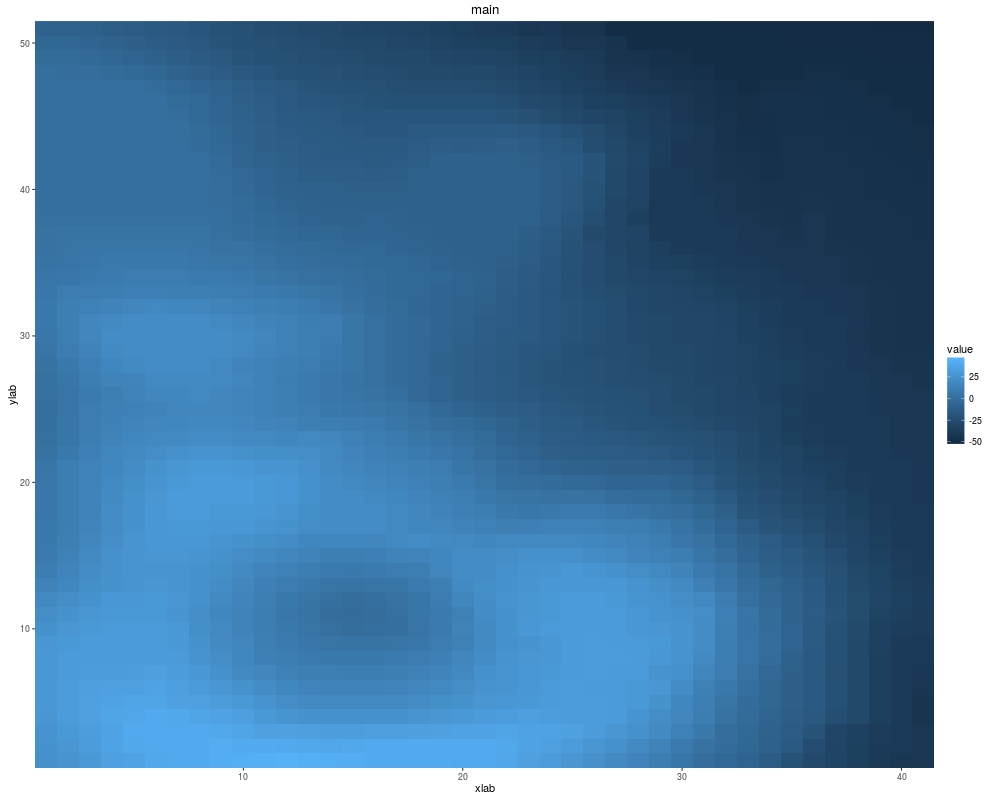
autoplot(volcano, xlab = "xlab", main = "main", ylab = "ylab")
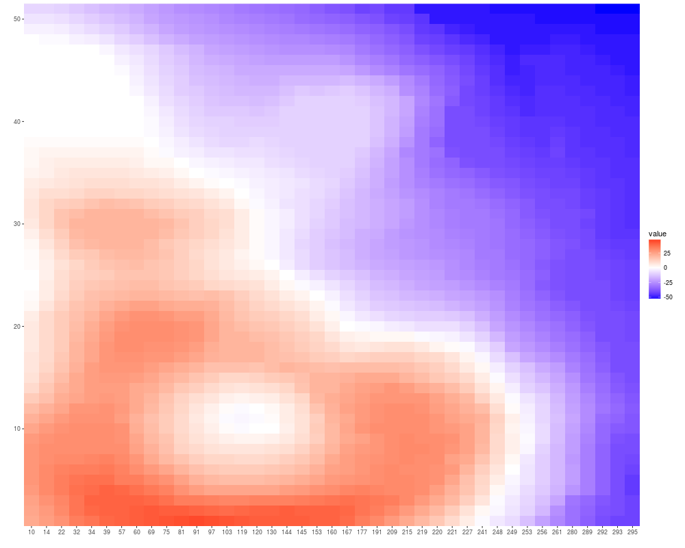
## special scale theme for 0-centered values
autoplot(volcano, geom = "raster")+scale_fill_fold_change()
## when a matrix has colnames and rownames label them by default
colnames(volcano) <- sort(sample(1:300, size = ncol(volcano), replace = FALSE))
autoplot(volcano)+scale_fill_fold_change()
rownames(volcano) <- letters[sample(1:24, size = nrow(volcano), replace = TRUE)]
autoplot(volcano)
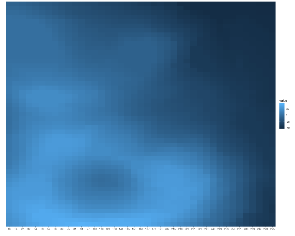
## even with row/col names, you could also disable it and just use numeric index
autoplot(volcano, colnames.label = FALSE)
autoplot(volcano, rownames.label = FALSE, colnames.label = FALSE)
## don't want the axis has label??
autoplot(volcano, axis.text.x = FALSE)
autoplot(volcano, axis.text.y = FALSE)
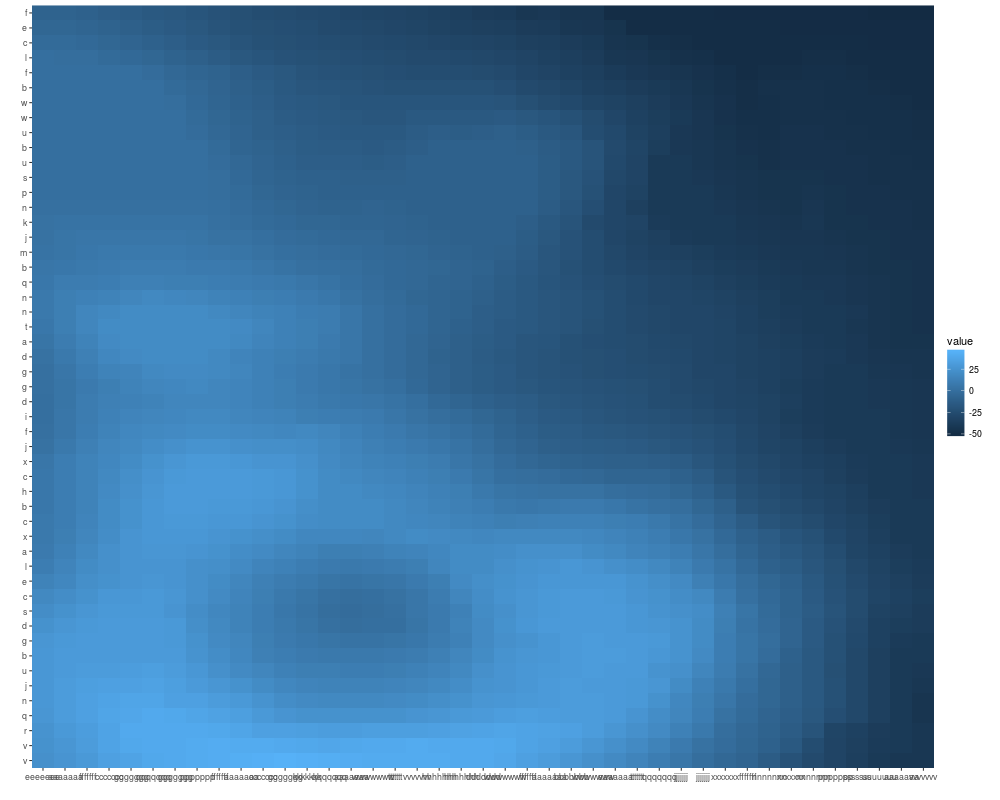
# or totally remove axis
colnames(volcano) <- lapply(letters[sample(1:24, size = ncol(volcano),
replace = TRUE)],
function(x){
paste(rep(x, 7), collapse = "")
})
## Oops, overlapped
autoplot(volcano)
## tweak with it.
autoplot(volcano, axis.text.angle = -45, hjust = 0)
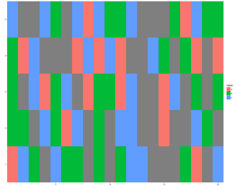
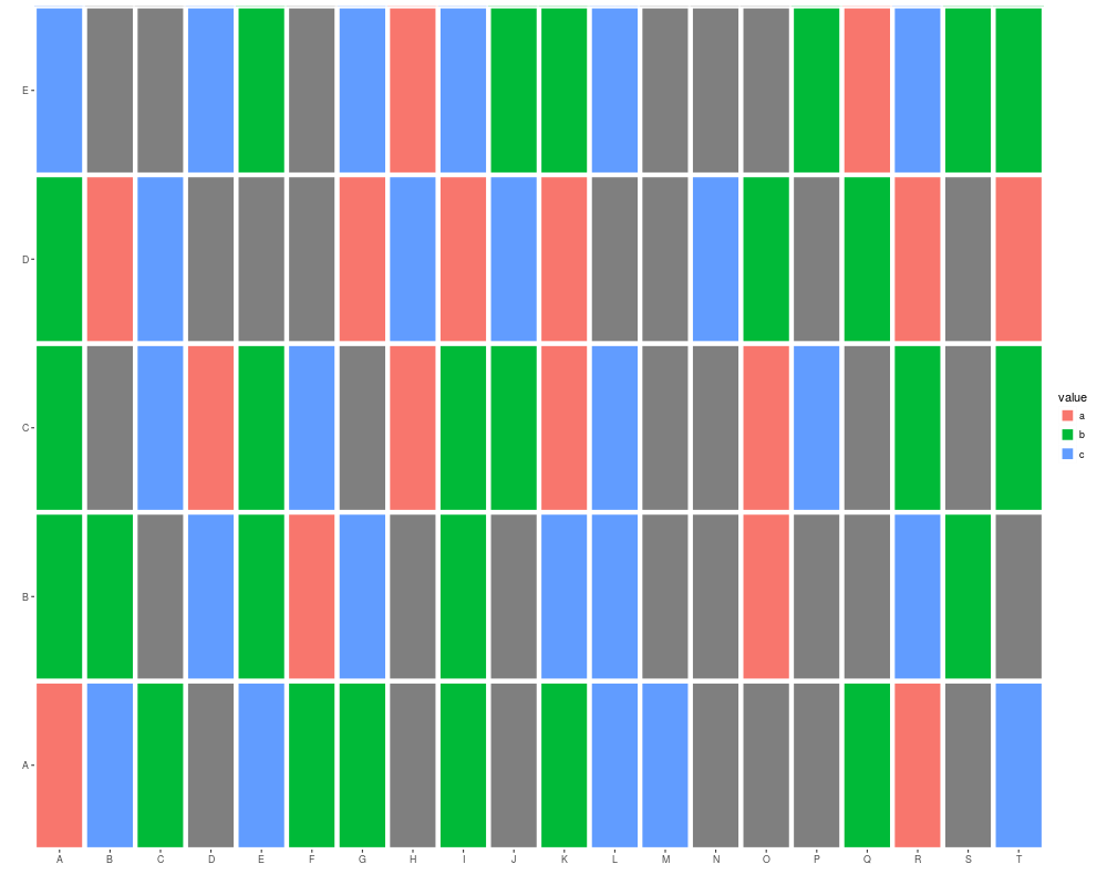
## when character is the value
x <- sample(c(letters[1:3], NA), size = 100, replace = TRUE)
mx <- matrix(x, nrow = 5)
autoplot(mx)
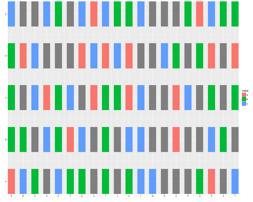
## tile gives you a white margin
rownames(mx) <- LETTERS[1:5]
autoplot(mx, color = "white")
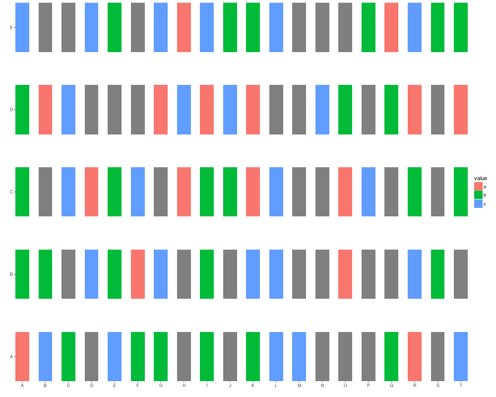
colnames(mx) <- LETTERS[1:20]
autoplot(mx, color = "white")
autoplot(mx, color = "white", size = 2)
## weird in aes(), though works
## default tile is flexible
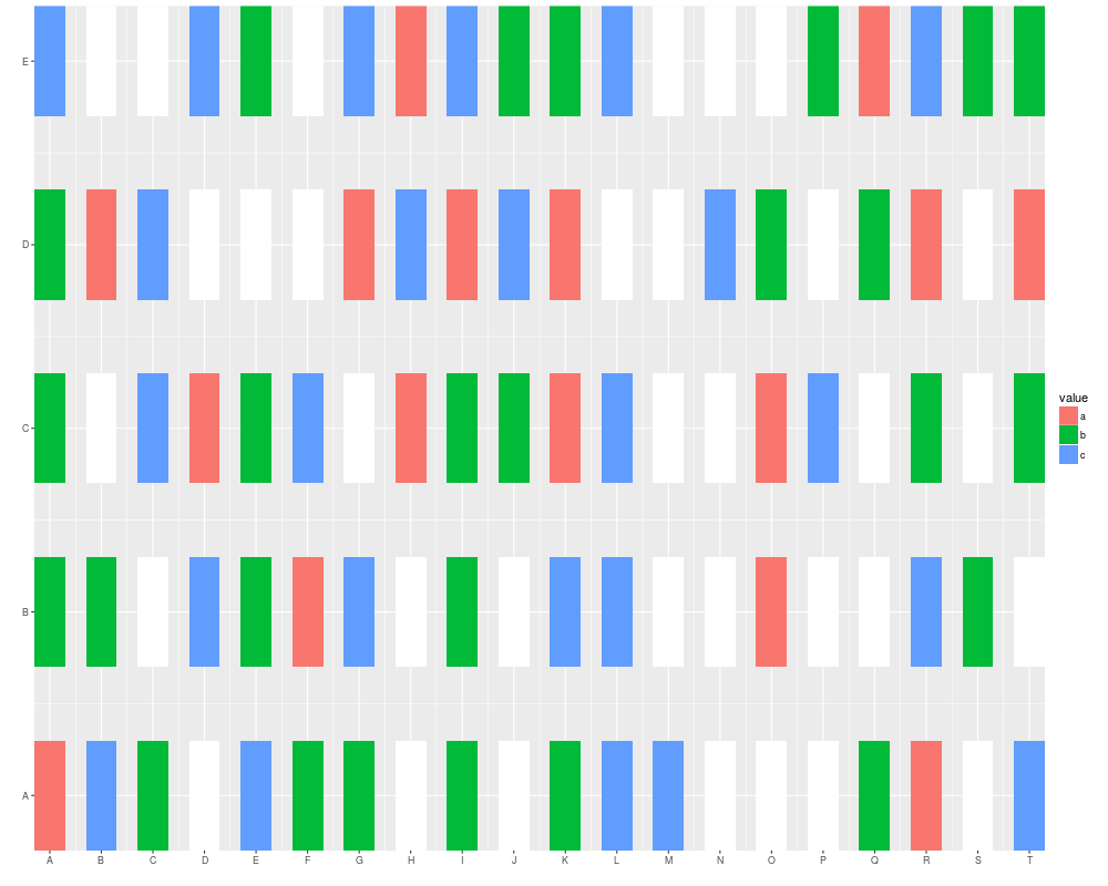
autoplot(mx, aes(width = 0.6, height = 0.6))
autoplot(mx, aes(width = 0.6, height = 0.6), na.value = "white")
autoplot(mx, aes(width = 0.6, height = 0.6)) + theme_clear()
###################################################
### Views
###################################################
lambda <- c(rep(0.001, 4500), seq(0.001, 10, length = 500),
seq(10, 0.001, length = 500))
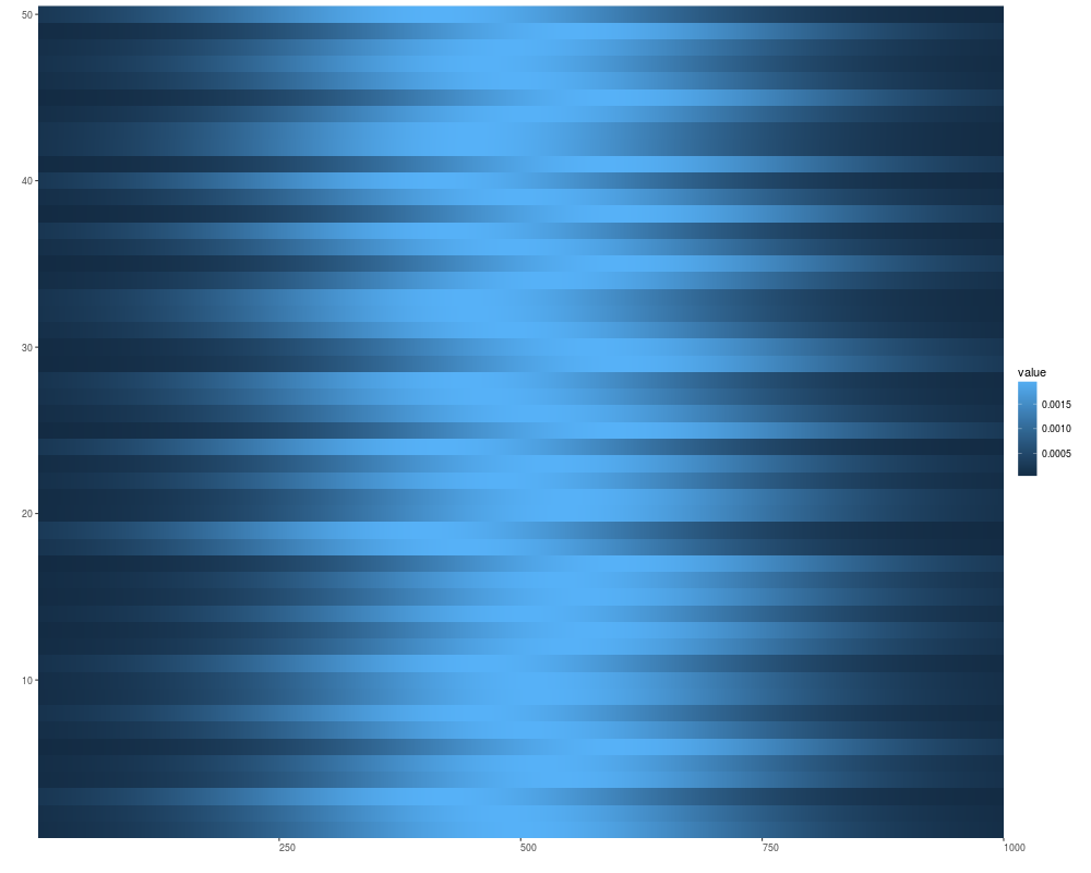
xVector <- dnorm(1:5e3, mean = 1e3, sd = 200)
xRle <- Rle(xVector)
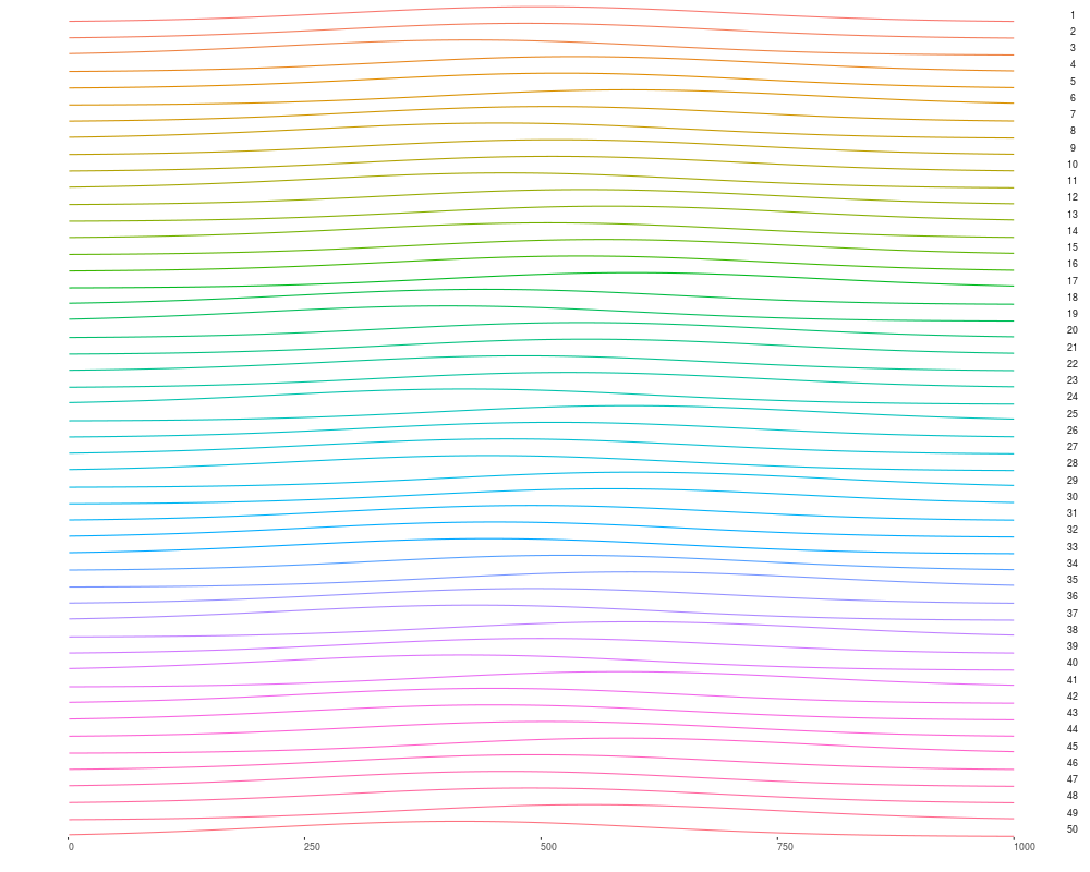
v1 <- Views(xRle, start = sample(.4e3:.6e3, size = 50, replace = FALSE), width =1000)
autoplot(v1)
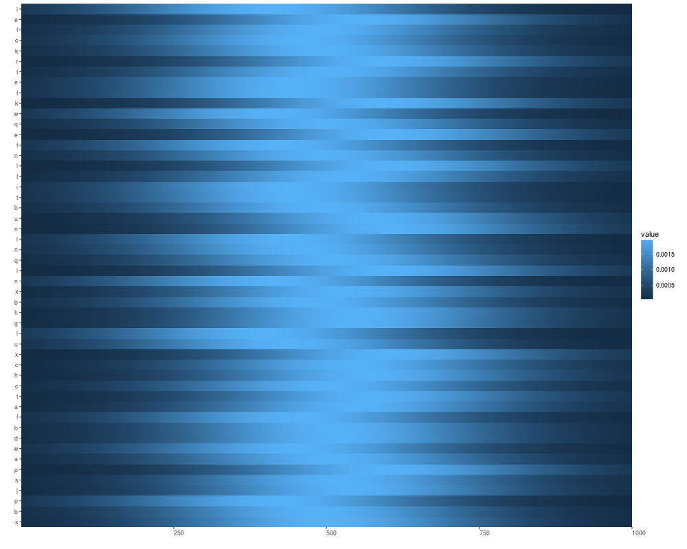
names(v1) <- letters[sample(1:24, size = length(v1), replace = TRUE)]
autoplot(v1)
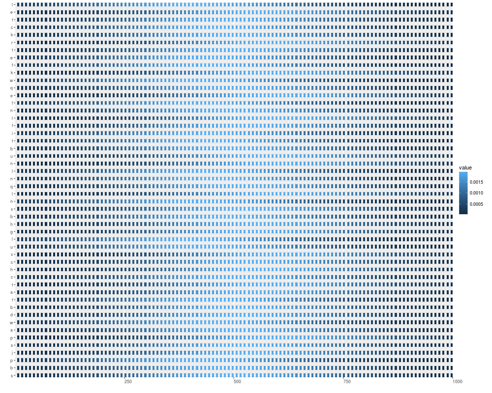
autoplot(v1, geom = "tile", aes(width = 0.5, height = 0.5))
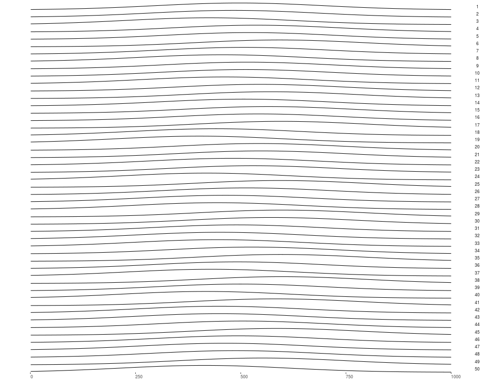
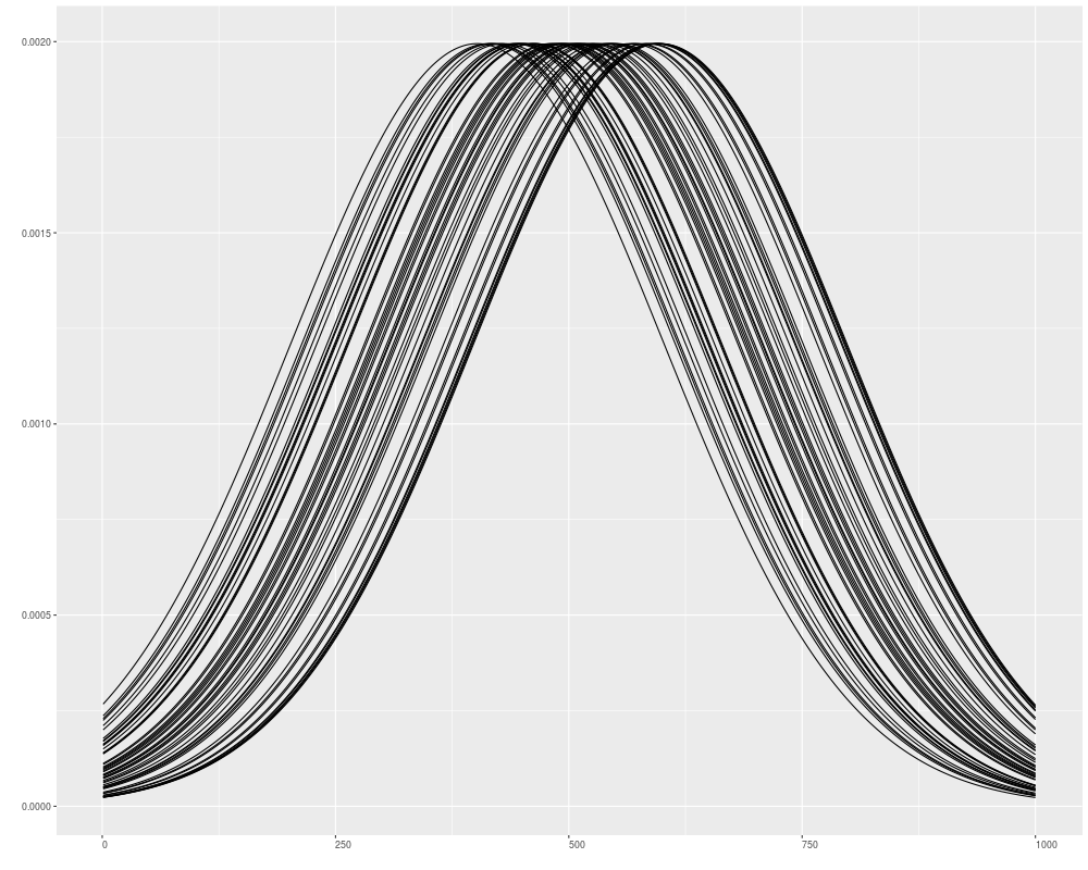
autoplot(v1, geom = "line")
autoplot(v1, geom = "line", aes(color = row)) + theme(legend.position = "none")
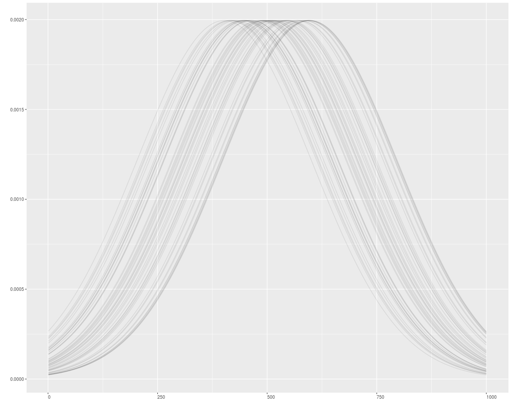
autoplot(v1, geom = "line", facets = NULL)
autoplot(v1, geom = "line", facets = NULL, alpha = 0.1)
###################################################
### ExpressionSet
###################################################
library(Biobase)
data(sample.ExpressionSet)
sample.ExpressionSet
set.seed(1)
## select 50 features
idx <- sample(seq_len(dim(sample.ExpressionSet)[1]), size = 50)
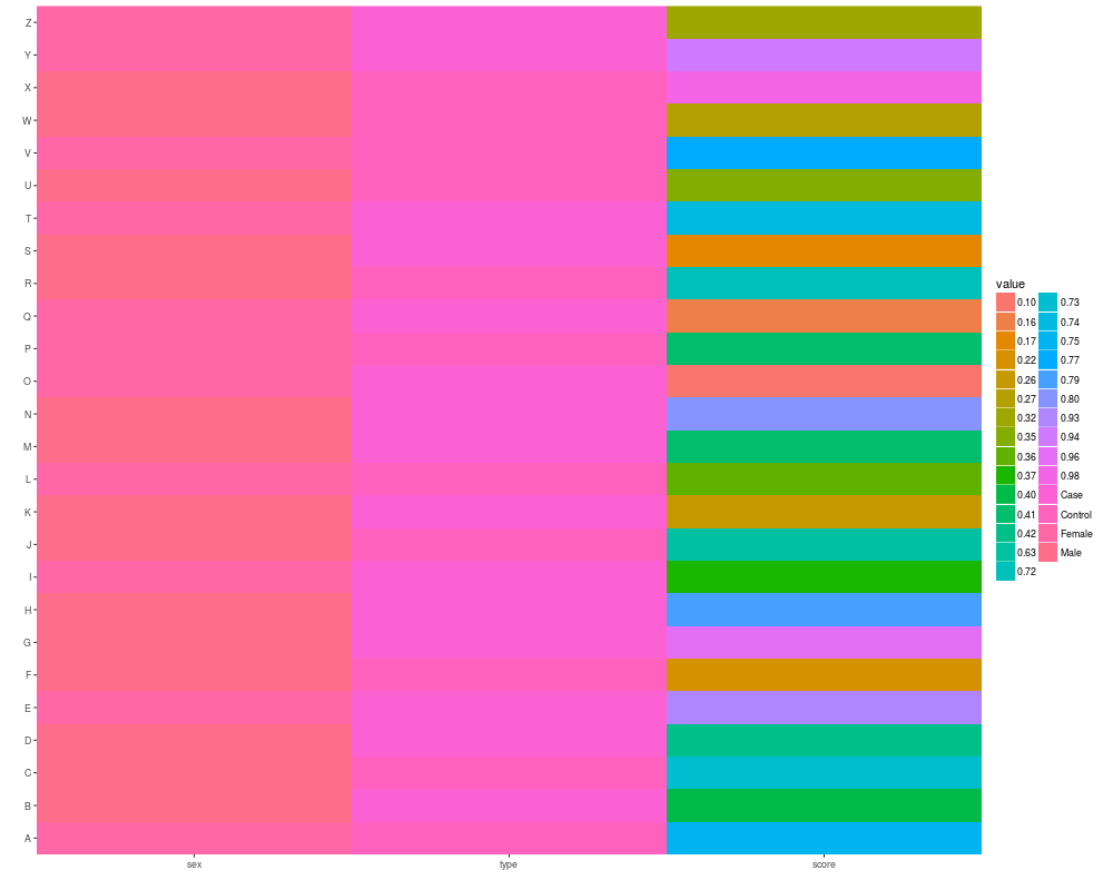
eset <- sample.ExpressionSet[idx,]
eset
autoplot(as.matrix(pData(eset)))
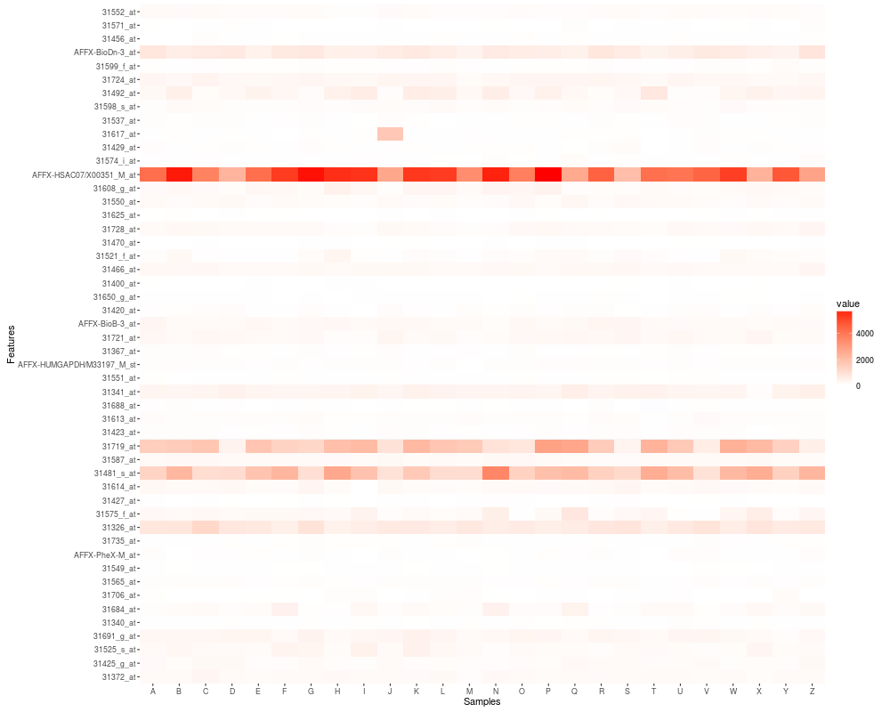
## default heatmap
p1 <- autoplot(eset)
p2 <- p1 + scale_fill_fold_change()
p2
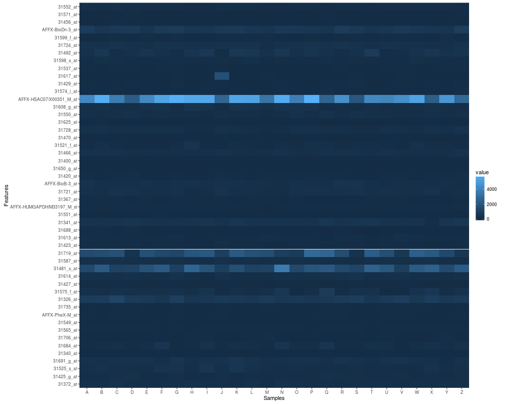
autoplot(eset)
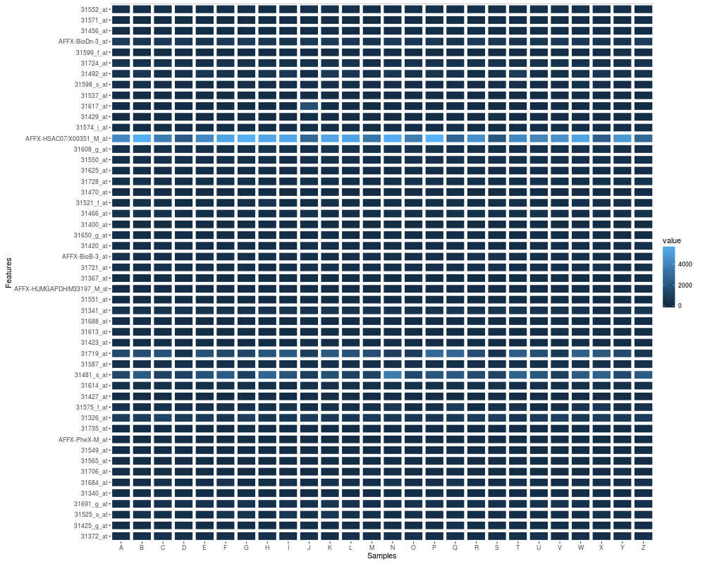
autoplot(eset, geom = "tile", color = "white", size = 2)
autoplot(eset, geom = "tile", aes(width = 0.6, height = 0.6))
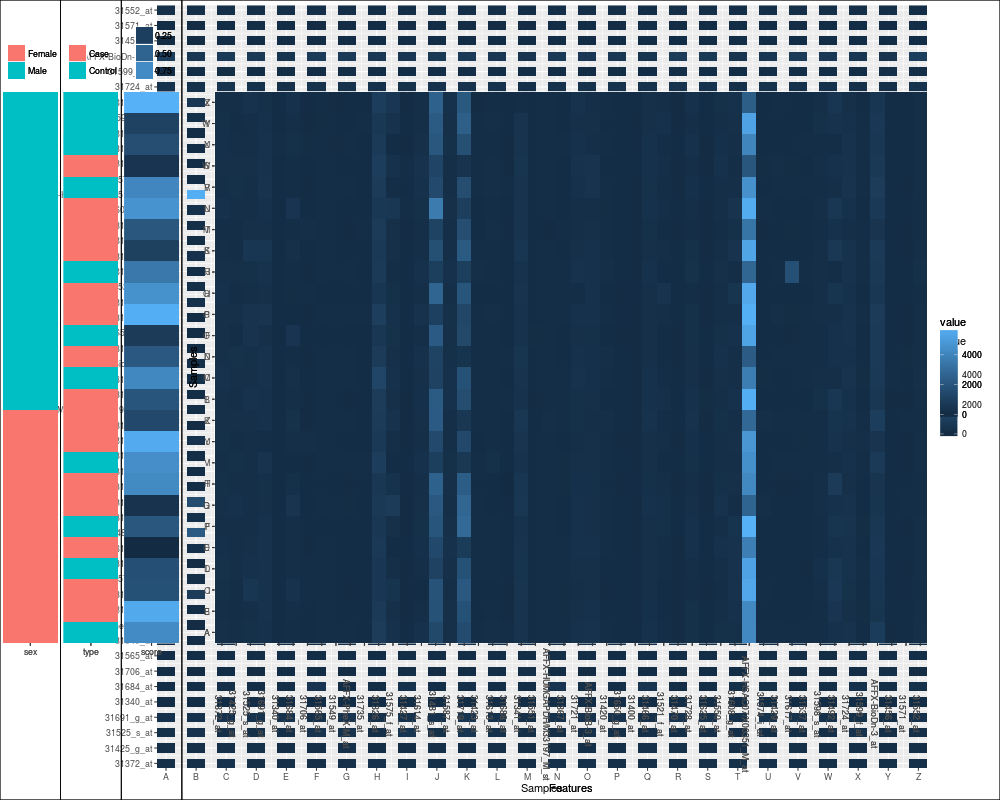
autoplot(eset, pheno.plot = TRUE)
idx <- order(pData(eset)[,1])
eset2 <- eset[,idx]
autoplot(eset2, pheno.plot = TRUE)
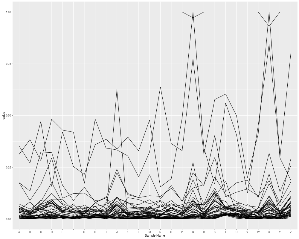
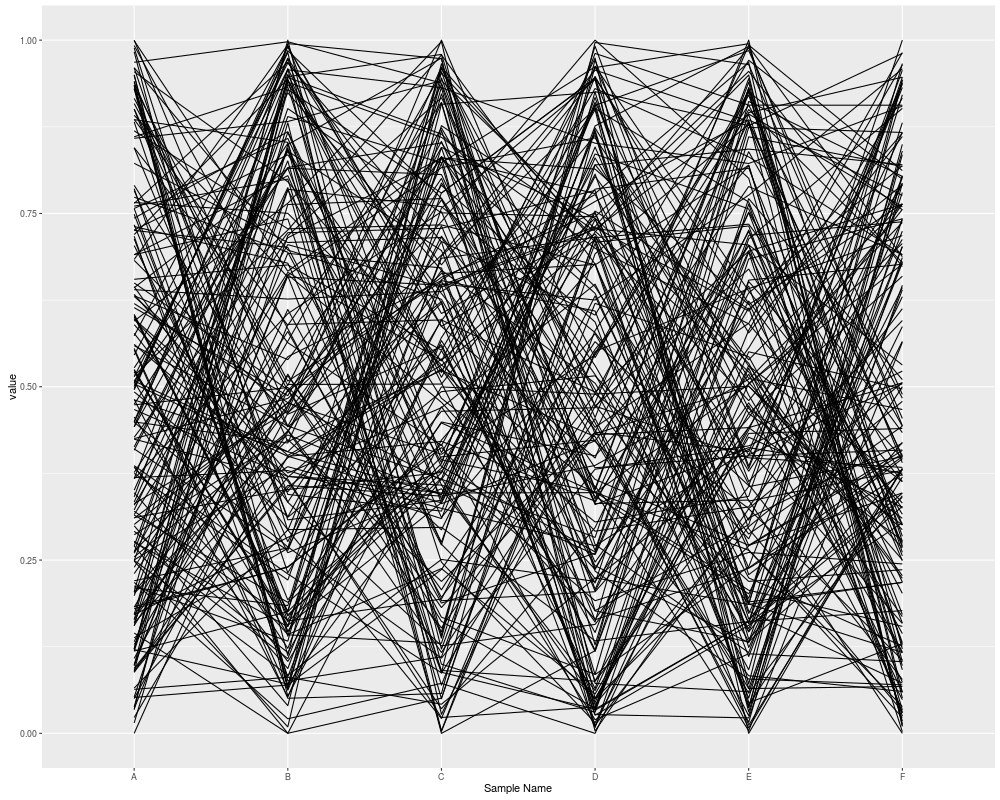
## parallel coordainte plot
autoplot(eset, type = "pcp")
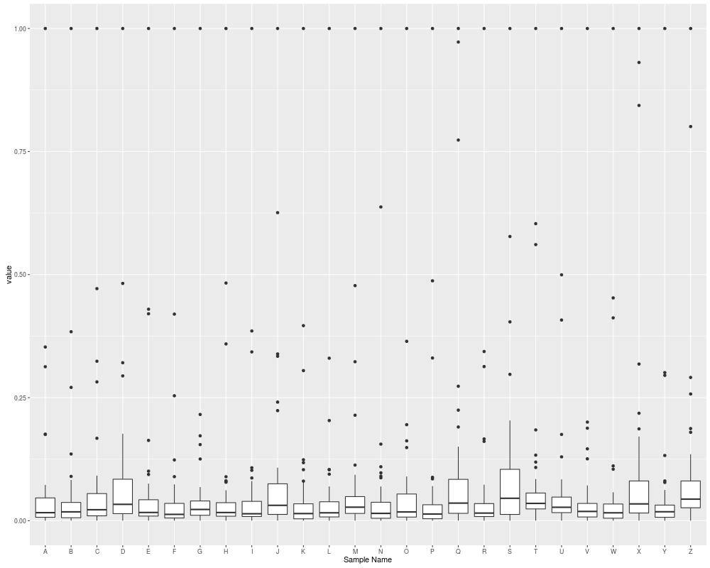
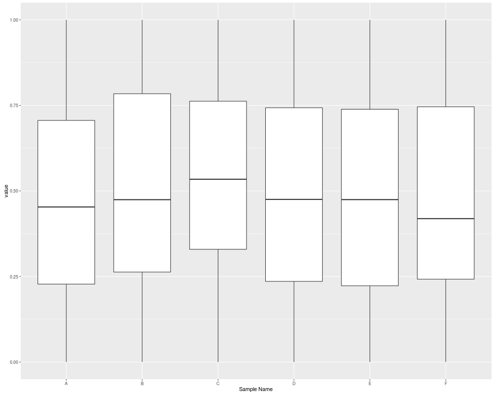
## boxplot
autoplot(eset, type = "boxplot")
## scatterplot.matrix
## slow, be carefull
##autoplot(eset[, 1:7], type = "scatterplot.matrix")
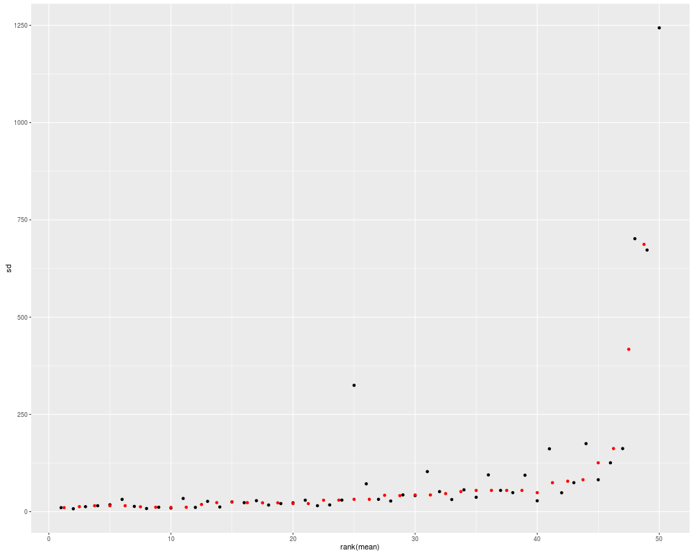
## mean-sd
autoplot(eset, type = "mean-sd")
###################################################
### RangedSummarizedExperiment
###################################################
library(SummarizedExperiment)
nrows <- 200; ncols <- 6
counts <- matrix(runif(nrows * ncols, 1, 1e4), nrows)
counts2 <- matrix(runif(nrows * ncols, 1, 1e4), nrows)
rowRanges <- GRanges(rep(c("chr1", "chr2"), c(50, 150)),
IRanges(floor(runif(200, 1e5, 1e6)), width=100),
strand=sample(c("+", "-"), 200, TRUE))
colData <- DataFrame(Treatment=rep(c("ChIP", "Input"), 3),
row.names=LETTERS[1:6])
sset <- SummarizedExperiment(assays=SimpleList(counts=counts,
counts2 = counts2),
rowRanges=rowRanges, colData=colData)
autoplot(sset) + scale_fill_fold_change()
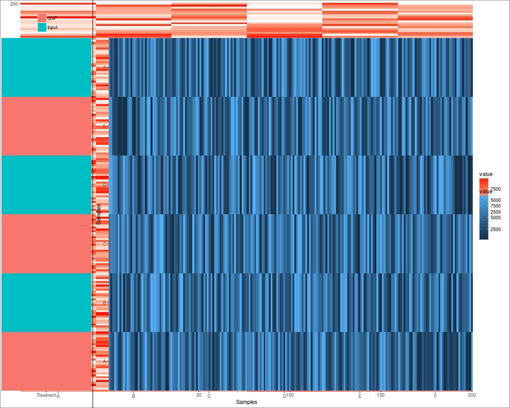
autoplot(sset, pheno.plot = TRUE)
###################################################
### pcp
###################################################
autoplot(sset, type = "pcp")
###################################################
### boxplot
###################################################
autoplot(sset, type = "boxplot")
###################################################
### scatterplot matrix
###################################################
##autoplot(sset, type = "scatterplot.matrix")
###################################################
### vcf
###################################################
## Not run:
library(VariantAnnotation)
vcffile <- system.file("extdata", "chr22.vcf.gz", package="VariantAnnotation")
vcf <- readVcf(vcffile, "hg19")
## default use type 'geno'
## default use genome position
autoplot(vcf)
## or disable it
autoplot(vcf, genome.axis = FALSE)
## not transpose
autoplot(vcf, genome.axis = FALSE, transpose = FALSE, rownames.label = FALSE)
autoplot(vcf)
## use
autoplot(vcf, assay.id = "DS")
## equivalent to
autoplot(vcf, assay.id = 2)
## doesn't work when assay.id cannot find
autoplot(vcf, assay.id = "NO")
## use AF or first
autoplot(vcf, type = "info")
## geom bar
autoplot(vcf, type = "info", aes(y = THETA))
autoplot(vcf, type = "info", aes(y = THETA, fill = VT, color = VT))
autoplot(vcf, type = "fixed")
autoplot(vcf, type = "fixed", size = 10) + xlim(c(50310860, 50310890)) + ylim(0.75, 1.25)
p1 <- autoplot(vcf, type = "fixed") + xlim(50310860, 50310890)
p2 <- autoplot(vcf, type = "fixed", full.string = TRUE) + xlim(50310860, 50310890)
tracks("full.string = FALSE" = p1, "full.string = TRUE" = p2)+
scale_y_continuous(breaks = NULL, limits = c(0, 3))
p3 <- autoplot(vcf, type = "fixed", ref.show = FALSE) + xlim(50310860, 50310890) +
scale_y_continuous(breaks = NULL, limits = c(0, 2))
p3
## End(Not run)
###################################################
### code chunk number 56: bs-v
###################################################
library(BSgenome.Hsapiens.UCSC.hg19)
data(genesymbol, package = "biovizBase")
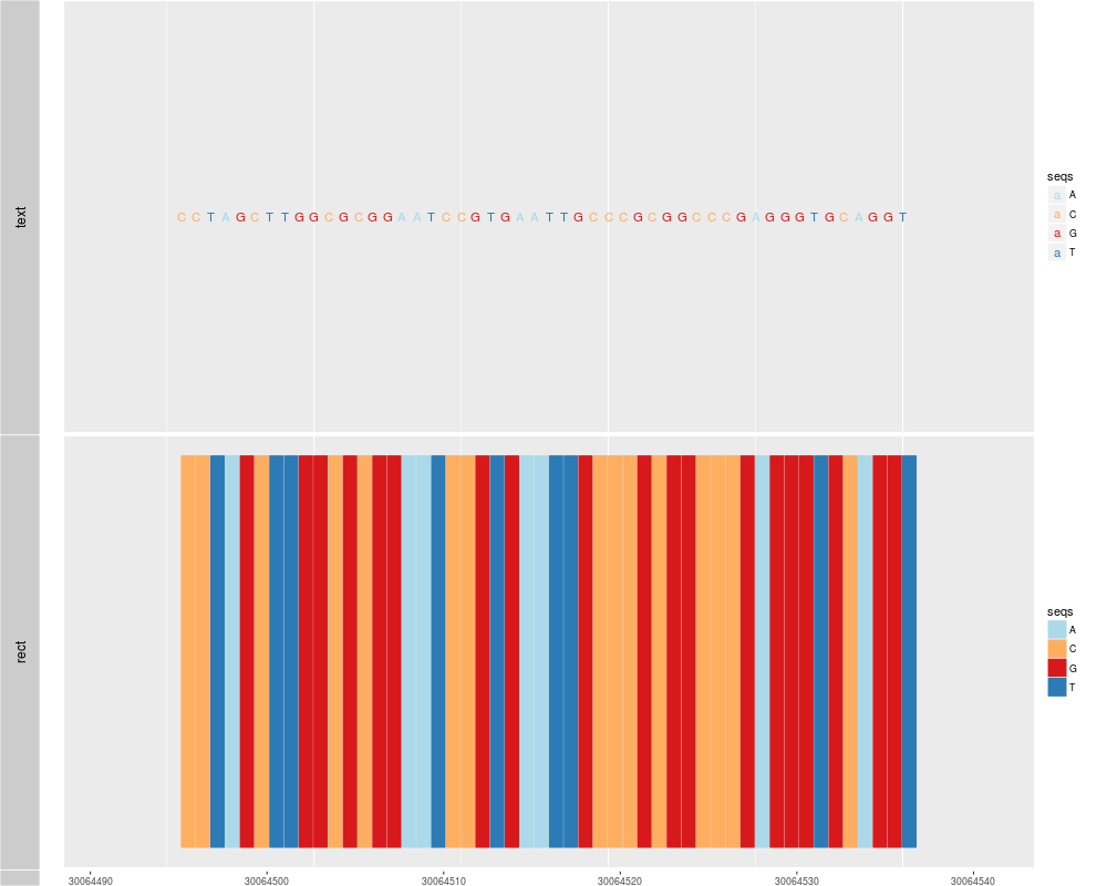
p1 <- autoplot(Hsapiens, which = resize(genesymbol["ALDOA"], width = 50))
p2 <- autoplot(Hsapiens, which = resize(genesymbol["ALDOA"], width = 50), geom = "rect")
tracks(text = p1, rect = p2)
###################################################
### code chunk number 57: sessionInfo
###################################################
sessionInfo()
Results
R version 3.3.1 (2016-06-21) -- "Bug in Your Hair"
Copyright (C) 2016 The R Foundation for Statistical Computing
Platform: x86_64-pc-linux-gnu (64-bit)

R is free software and comes with ABSOLUTELY NO WARRANTY.
You are welcome to redistribute it under certain conditions.
Type 'license()' or 'licence()' for distribution details.

R is a collaborative project with many contributors.
Type 'contributors()' for more information and
'citation()' on how to cite R or R packages in publications.

Type 'demo()' for some demos, 'help()' for on-line help, or
'help.start()' for an HTML browser interface to help.
Type 'q()' to quit R.

> library(ggbio)
Loading required package: BiocGenerics
Loading required package: parallel

Attaching package: 'BiocGenerics'

The following objects are masked from 'package:parallel':

    clusterApply, clusterApplyLB, clusterCall, clusterEvalQ,
    clusterExport, clusterMap, parApply, parCapply, parLapply,
    parLapplyLB, parRapply, parSapply, parSapplyLB

The following objects are masked from 'package:stats':

    IQR, mad, xtabs

The following objects are masked from 'package:base':

    Filter, Find, Map, Position, Reduce, anyDuplicated, append,
    as.data.frame, cbind, colnames, do.call, duplicated, eval, evalq,
    get, grep, grepl, intersect, is.unsorted, lapply, lengths, mapply,
    match, mget, order, paste, pmax, pmax.int, pmin, pmin.int, rank,
    rbind, rownames, sapply, setdiff, sort, table, tapply, union,
    unique, unsplit

Loading required package: ggplot2
Need specific help about ggbio? try mailing
 the maintainer or visit http://tengfei.github.com/ggbio/

Attaching package: 'ggbio'

The following objects are masked from 'package:ggplot2':

    geom_bar, geom_rect, geom_segment, ggsave, stat_bin, stat_identity,
    xlim

Warning message:
replacing previous import 'ggplot2::Position' by 'BiocGenerics::Position' when loading 'ggbio'
> png(filename="/home/ddbj/snapshot/RGM3/R_BC/result/ggbio/autoplot-method.Rd_%03d_medium.png", width=480, height=480)
> ### Name: autoplot
> ### Title: Generic autoplot function
> ### Aliases: autoplot autoplot,GRanges-method autoplot,GRangesList-method
> ###   autoplot,IRanges-method autoplot,Seqinfo-method
> ###   autoplot,BSgenome-method autoplot,GAlignments-method
> ###   autoplot,BamFile-method autoplot,BamFileList-method
> ###   autoplot,TxDbOREnsDb-method autoplot,character-method
> ###   autoplot,Rle-method autoplot,RleList-method autoplot,matrix-method
> ###   autoplot,Views-method autoplot,ExpressionSet-method
> ###   autoplot,RangedSummarizedExperiment-method autoplot,VCF-method
> ###   autoplot,OrganismDb-method autoplot,VRanges-method
> ###   autoplot,TabixFile-method +,Bioplot,Any-method
>
> ### ** Examples
>
> library(ggbio)
>
> set.seed(1)
> N <- 1000
> library(GenomicRanges)
Loading required package: S4Vectors
Loading required package: stats4

Attaching package: 'S4Vectors'

The following objects are masked from 'package:base':

    colMeans, colSums, expand.grid, rowMeans, rowSums

Loading required package: IRanges
Loading required package: GenomeInfoDb
> gr <- GRanges(seqnames =
+               sample(c("chr1", "chr2", "chr3"),
+                      size = N, replace = TRUE),
+               IRanges(
+                       start = sample(1:300, size = N, replace = TRUE),
+                       width = sample(70:75, size = N,replace = TRUE)),
+               strand = sample(c("+", "-", "*"), size = N,
+                 replace = TRUE),
+               value = rnorm(N, 10, 3), score = rnorm(N, 100, 30),
+               sample = sample(c("Normal", "Tumor"),
+                 size = N, replace = TRUE),
+               pair = sample(letters, size = N,
+                 replace = TRUE))
>
> idx <- sample(1:length(gr), size = 50)
>
>
> ###################################################
> ### code chunk number 3: default
> ###################################################
> autoplot(gr[idx])
>
>
> ###################################################
> ### code chunk number 4: bar-default-pre
> ###################################################
> set.seed(123)
> gr.b <- GRanges(seqnames = "chr1", IRanges(start = seq(1, 100, by = 10),
+                   width = sample(4:9, size = 10, replace = TRUE)),
+                 score = rnorm(10, 10, 3), value = runif(10, 1, 100))
> gr.b2 <- GRanges(seqnames = "chr2", IRanges(start = seq(1, 100, by = 10),
+                   width = sample(4:9, size = 10, replace = TRUE)),
+                 score = rnorm(10, 10, 3), value = runif(10, 1, 100))
> gr.b <- c(gr.b, gr.b2)
Warning message:
In .Seqinfo.mergexy(x, y) :
  The 2 combined objects have no sequence levels in common. (Use
  suppressWarnings() to suppress this warning.)
> head(gr.b)
GRanges object with 6 ranges and 2 metadata columns:
      seqnames    ranges strand |            score            value
         <Rle> <IRanges>  <Rle> |        <numeric>        <numeric>
  [1]     chr1  [ 1,  9]      * | 8.31857306034336 89.0643922903109
  [2]     chr1  [11, 19]      * | 9.30946753155016 69.5875372095034
  [3]     chr1  [21, 28]      * | 14.6761249424474 64.4101745630614
  [4]     chr1  [31, 38]      * | 10.2115251742737 99.4327078857459
  [5]     chr1  [41, 44]      * | 10.3878632054828 65.9148741124664
  [6]     chr1  [51, 56]      * | 15.1451949606498  71.144516348606
  -------
  seqinfo: 2 sequences from an unspecified genome; no seqlengths
>
>
> ###################################################
> ### code chunk number 5: bar-default
> ###################################################
> p1 <- autoplot(gr.b, geom = "bar")
use score as y by default
> ## use value to fill the bar
> p2 <- autoplot(gr.b, geom = "bar", aes(fill = value))
use score as y by default
> tracks(default = p1, fill = p2)
>
>
> ###################################################
> ### code chunk number 6: autoplot.Rnw:236-237
> ###################################################
> autoplot(gr[idx], geom = "arch", aes(color = value), facets = sample ~ seqnames)
>
>
> ###################################################
> ### code chunk number 7: gr-group
> ###################################################
> gra <- GRanges("chr1", IRanges(c(1,7,20), end = c(4,9,30)), group = c("a", "a", "b"))
> ## if you desn't specify group, then group based on stepping levels, and gaps are computed without
> ## considering extra group method
> p1 <- autoplot(gra, aes(fill = group), geom = "alignment")
> ## when use group method, gaps only computed for grouped intervals.
> ## default is group.selfish = TRUE, each group keep one row.
> ## in this way, group labels could be shown as y axis.
> p2 <- autoplot(gra, aes(fill = group, group = group), geom = "alignment")
> ## group.selfish = FALSE, save space
> p3 <- autoplot(gra, aes(fill = group, group = group), geom = "alignment", group.selfish = FALSE)
> tracks('non-group' = p1,'group.selfish = TRUE' = p2 , 'group.selfish = FALSE' = p3)
>
>
> ###################################################
> ### code chunk number 8: gr-facet-strand
> ###################################################
> autoplot(gr, stat = "coverage", geom = "area",
+          facets = strand ~ seqnames, aes(fill = strand))
Scale for 'x' is already present. Adding another scale for 'x', which will
replace the existing scale.
>
>
> ###################################################
> ### code chunk number 9: gr-autoplot-circle
> ###################################################
> autoplot(gr[idx], layout = 'circle')
>
>
> ###################################################
> ### code chunk number 10: gr-circle
> ###################################################
> seqlengths(gr) <- c(400, 500, 700)
> values(gr)$to.gr <- gr[sample(1:length(gr), size = length(gr))]
> idx <- sample(1:length(gr), size = 50)
> gr <- gr[idx]
> ggplot() + layout_circle(gr, geom = "ideo", fill = "gray70", radius = 7, trackWidth = 3) +
+   layout_circle(gr, geom = "bar", radius = 10, trackWidth = 4,
+                 aes(fill = score, y = score)) +
+   layout_circle(gr, geom = "point", color = "red", radius = 14,
+                 trackWidth = 3, grid = TRUE, aes(y = score)) +
+   layout_circle(gr, geom = "link", linked.to = "to.gr", radius = 6, trackWidth = 1)
>
>
> ###################################################
> ### code chunk number 11: seqinfo-src
> ###################################################
> data(hg19Ideogram, package = "biovizBase")
> sq <- seqinfo(hg19Ideogram)
> sq
Seqinfo object with 93 sequences from hg19 genome:
  seqnames             seqlengths isCircular genome
  chr1                  249250621       <NA>   hg19
  chr1_gl000191_random     106433       <NA>   hg19
  chr1_gl000192_random     547496       <NA>   hg19
  chr2                  243199373       <NA>   hg19
  chr3                  198022430       <NA>   hg19
  ...                         ...        ...    ...
  chrUn_gl000246            38154       <NA>   hg19
  chrUn_gl000247            36422       <NA>   hg19
  chrUn_gl000248            39786       <NA>   hg19
  chrUn_gl000249            38502       <NA>   hg19
  chrM                      16571       <NA>   hg19
>
>
> ###################################################
> ### code chunk number 12: seqinfo
> ###################################################
> autoplot(sq[paste0("chr", c(1:22, "X"))])
>
>
> ###################################################
> ### code chunk number 13: ir-load
> ###################################################
> set.seed(1)
> N <- 100
> ir <-  IRanges(start = sample(1:300, size = N, replace = TRUE),
+                width = sample(70:75, size = N,replace = TRUE))
> ## add meta data
> df <- DataFrame(value = rnorm(N, 10, 3), score = rnorm(N, 100, 30),
+               sample = sample(c("Normal", "Tumor"),
+                 size = N, replace = TRUE),
+               pair = sample(letters, size = N,
+                 replace = TRUE))
> values(ir) <- df
> ir
IRanges object with 100 ranges and 4 metadata columns:
            start       end     width |     value     score      sample
        <integer> <integer> <integer> | <numeric> <numeric> <character>
    [1]        80       152        73 |  8.138900 112.28206       Tumor
    [2]       112       183        72 | 10.126348 150.66620       Tumor
    [3]       172       242        71 |  7.267235 147.59765      Normal
    [4]       273       347        75 | 10.474086  90.07277       Tumor
    [5]        61       133        73 |  8.036246  31.44293       Tumor
    ...       ...       ...       ... .       ...       ...         ...
   [96]       240       312        73 |  6.856047 104.03343       Tumor
   [97]       137       206        70 | 14.323473 122.96797       Tumor
   [98]       124       198        75 |  6.952458 128.65410      Normal
   [99]       244       314        71 | 11.235924  98.48303       Tumor
  [100]       182       255        74 |  8.856772  90.82554      Normal
               pair
        <character>
    [1]           y
    [2]           x
    [3]           t
    [4]           r
    [5]           q
    ...         ...
   [96]           q
   [97]           g
   [98]           n
   [99]           u
  [100]           j
>
>
> ###################################################
> ### code chunk number 14: ir-exp
> ###################################################
> p1 <- autoplot(ir)
> p2 <- autoplot(ir, aes(fill = pair)) + theme(legend.position = "none")
> p3 <- autoplot(ir, stat = "coverage", geom = "line", facets = sample ~. )
Scale for 'x' is already present. Adding another scale for 'x', which will
replace the existing scale.
> p4 <- autoplot(ir, stat = "reduce")
Scale for 'x' is already present. Adding another scale for 'x', which will
replace the existing scale.
> tracks(p1, p2, p3, p4)
>
>
> ###################################################
> ### code chunk number 15: grl-simul
> ###################################################
> set.seed(1)
> N <- 100
> ## ======================================================================
> ##  simmulated GRanges
> ## ======================================================================
> gr <- GRanges(seqnames =
+               sample(c("chr1", "chr2", "chr3"),
+                      size = N, replace = TRUE),
+               IRanges(
+                       start = sample(1:300, size = N, replace = TRUE),
+                       width = sample(30:40, size = N,replace = TRUE)),
+               strand = sample(c("+", "-", "*"), size = N,
+                 replace = TRUE),
+               value = rnorm(N, 10, 3), score = rnorm(N, 100, 30),
+               sample = sample(c("Normal", "Tumor"),
+                 size = N, replace = TRUE),
+               pair = sample(letters, size = N,
+                 replace = TRUE))
>
>
> grl <- split(gr, values(gr)$pair)
>
>
> ###################################################
> ### code chunk number 16: grl-exp
> ###################################################
> ## default gap.geom is 'chevron'
> p1 <- autoplot(grl, group.selfish = TRUE)
> p2 <- autoplot(grl, group.selfish = TRUE, main.geom = "arrowrect", gap.geom = "segment")
> tracks(p1, p2)
>
>
> ###################################################
> ### code chunk number 17: grl-name
> ###################################################
> autoplot(grl, aes(fill = ..grl_name..))
> ## equal to
> ## autoplot(grl, aes(fill = grl_name))
>
>
> ###################################################
> ### code chunk number 18: rle-simul
> ###################################################
> library(IRanges)
> set.seed(1)
> lambda <- c(rep(0.001, 4500), seq(0.001, 10, length = 500),
+             seq(10, 0.001, length = 500))
>
> ## @knitr create
> xVector <- rpois(1e4, lambda)
> xRle <- Rle(xVector)
> xRle
integer-Rle of length 10000 with 823 runs
  Lengths:  779    1  208    1 1599    1  883 ...    1    5    2    9    1 4507
  Values :    0    1    0    1    0    1    0 ...    1    0    1    0    1    0
>
>
> ###################################################
> ### code chunk number 19: rle-bin
> ###################################################
> p1 <- autoplot(xRle)
Default use binwidth: range/30
> p2 <- autoplot(xRle, nbin = 80)
Default use binwidth: range/80
> p3 <- autoplot(xRle, geom = "heatmap", nbin = 200)
Default use binwidth: range/200
> tracks('nbin = 30' = p1, "nbin = 80" = p2, "nbin = 200(heatmap)" = p3)
>
>
> ###################################################
> ### code chunk number 20: rle-id
> ###################################################
> p1 <- autoplot(xRle, stat = "identity")
> p2 <- autoplot(xRle, stat = "identity", geom = "point", color = "red")
> tracks('line' = p1, "point" = p2)
>
>
> ###################################################
> ### code chunk number 21: rle-slice
> ###################################################
> p1 <- autoplot(xRle, type = "viewMaxs", stat = "slice", lower = 5)
> p2 <- autoplot(xRle, type = "viewMaxs", stat = "slice", lower = 5, geom = "heatmap")
> tracks('bar' = p1, "heatmap" = p2)
>
>
> ###################################################
> ### code chunk number 22: rlel-simul
> ###################################################
> xRleList <- RleList(xRle, 2L * xRle)
> xRleList
RleList of length 2
[[1]]
integer-Rle of length 10000 with 823 runs
  Lengths:  779    1  208    1 1599    1  883 ...    1    5    2    9    1 4507
  Values :    0    1    0    1    0    1    0 ...    1    0    1    0    1    0

[[2]]
integer-Rle of length 10000 with 823 runs
  Lengths:  779    1  208    1 1599    1  883 ...    1    5    2    9    1 4507
  Values :    0    2    0    2    0    2    0 ...    2    0    2    0    2    0

>
>
> ###################################################
> ### code chunk number 23: rlel-bin
> ###################################################
> p1 <- autoplot(xRleList)
Default use binwidth: range/30
> p2 <- autoplot(xRleList, nbin = 80)
Default use binwidth: range/80
> p3 <- autoplot(xRleList, geom = "heatmap", nbin = 200)
Default use binwidth: range/200
> tracks('nbin = 30' = p1, "nbin = 80" = p2, "nbin = 200(heatmap)" = p3)
>
>
> ###################################################
> ### code chunk number 24: rlel-id
> ###################################################
> p1 <- autoplot(xRleList, stat = "identity")
> p2 <- autoplot(xRleList, stat = "identity", geom = "point", color = "red")
> tracks('line' = p1, "point" = p2)
>
>
> ###################################################
> ### code chunk number 25: rlel-slice
> ###################################################
> p1 <- autoplot(xRleList, type = "viewMaxs", stat = "slice", lower = 5)
> p2 <- autoplot(xRleList, type = "viewMaxs", stat = "slice", lower = 5, geom = "heatmap")
> tracks('bar' = p1, "heatmap" = p2)
>
>
> ###################################################
> ### code chunk number 26: txdb
> ###################################################
> library(TxDb.Hsapiens.UCSC.hg19.knownGene)
Loading required package: GenomicFeatures
Loading required package: AnnotationDbi
Loading required package: Biobase
Welcome to Bioconductor

    Vignettes contain introductory material; view with
    'browseVignettes()'. To cite Bioconductor, see
    'citation("Biobase")', and for packages 'citation("pkgname")'.

> data(genesymbol, package = "biovizBase")
> txdb <- TxDb.Hsapiens.UCSC.hg19.knownGene
>
>
> ###################################################
> ### code chunk number 27: txdb-visual
> ###################################################
> p1 <- autoplot(txdb, which = genesymbol["ALDOA"], names.expr = "tx_name:::gene_id")
Parsing transcripts...
Parsing exons...
Parsing cds...
Parsing utrs...
------exons...
------cdss...
------introns...
------utr...
aggregating...
Done
"gap" not in any of the valid gene feature terms "cds", "exon", "utr"
Constructing graphics...
> p2 <- autoplot(txdb, which = genesymbol["ALDOA"], stat = "reduce", color = "brown",
+                fill = "brown")
Parsing transcripts...
Parsing exons...
Parsing cds...
Parsing utrs...
------exons...
------cdss...
------introns...
------utr...
aggregating...
Done
"gap" not in any of the valid gene feature terms "cds", "exon", "utr"
Constructing graphics...
reduce alignemnts...
> tracks(full = p1, reduce = p2, heights = c(5, 1)) + ylab("")
>
>
> ###################################################
> ### EnsDb
> ###################################################
> ## Fetching gene models from an EnsDb object.
> library(EnsDb.Hsapiens.v75)
Loading required package: ensembldb
> ensdb <- EnsDb.Hsapiens.v75
> ## We use a GenenameFilter to specifically retrieve all transcripts for that gene.
> p1 <- autoplot(ensdb, which=GenenameFilter("ALDOA"), names.expr="gene_name")
Fetching data...OK
Parsing exons...OK
Defining introns...OK
Defining UTRs...OK
Defining CDS...OK
aggregating...
Done
"gap" not in any of the valid gene feature terms "cds", "exon", "utr"
Constructing graphics...
> p2 <- autoplot(ensdb, which=GenenameFilter("ALDOA"), stat="reduce", color="brown",
+                fill="brown")
Fetching data...OK
Parsing exons...OK
Defining introns...OK
Defining UTRs...OK
Defining CDS...OK
aggregating...
Done
"gap" not in any of the valid gene feature terms "cds", "exon", "utr"
Constructing graphics...
reduce alignemnts...
> tracks(full = p1, reduce = p2, heights = c(5, 1)) + ylab("")
>
> ## Alternatively, we can specify a GRangesFilter and display all genes
> ## that are (partially) overlapping with that genomic region:
> gr <- GRanges(seqnames=16, IRanges(30768000, 30770000), strand="+")
> autoplot(ensdb, GRangesFilter(gr, "overlapping"), names.expr="gene_name")
Fetching data...OK
Parsing exons...OK
Defining introns...OK
Defining UTRs...OK
Defining CDS...OK
aggregating...
Done
"gap" not in any of the valid gene feature terms "cds", "exon", "utr"
Constructing graphics...
> ## Just submitting the GRanges object also works.
> autoplot(ensdb, gr, names.expr="gene_name")
Fetching data...OK
Parsing exons...OK
Defining introns...OK
Defining UTRs...OK
Defining CDS...OK
aggregating...
Done
"gap" not in any of the valid gene feature terms "cds", "exon", "utr"
Constructing graphics...
>
> ## Or genes encoded on both strands.
> gr <- GRanges(seqnames=16, IRanges(30768000, 30770000), strand="*")
> autoplot(ensdb, GRangesFilter(gr, "overlapping"), names.expr="gene_name")
Fetching data...OK
Parsing exons...OK
Defining introns...OK
Defining UTRs...OK
Defining CDS...OK
aggregating...
Done
"gap" not in any of the valid gene feature terms "cds", "exon", "utr"
Constructing graphics...
>
> ## Also, we can spefify directly the gene ids and plot all transcripts of these
> ## genes (not only those overlapping with the region)
> autoplot(ensdb, GeneidFilter(c("ENSG00000196118", "ENSG00000156873")))
Fetching data...OK
Parsing exons...OK
Defining introns...OK
Defining UTRs...OK
Defining CDS...OK
aggregating...
Done
"gap" not in any of the valid gene feature terms "cds", "exon", "utr"
Constructing graphics...
>
> ###################################################
> ### code chunk number 28: ga-load
> ###################################################
> library(GenomicAlignments)
Loading required package: SummarizedExperiment
Loading required package: Biostrings
Loading required package: XVector
Loading required package: Rsamtools
> data("genesymbol", package = "biovizBase")
> bamfile <- system.file("extdata", "SRR027894subRBM17.bam",
+                        package="biovizBase")
> which <- keepStandardChromosomes(genesymbol["RBM17"])
> ## need to set use.names = TRUE
> ga <- readGAlignments(bamfile,
+                       param = ScanBamParam(which = which),
+                       use.names = TRUE)
>
>
> ###################################################
> ### code chunk number 29: ga-exp
> ###################################################
> p1 <- autoplot(ga)
> p2 <- autoplot(ga, geom = "rect")
extracting information...
> p3 <- autoplot(ga, geom = "line", stat = "coverage")
extracting information...
Scale for 'x' is already present. Adding another scale for 'x', which will
replace the existing scale.
> tracks(default = p1, rect = p2, coverage = p3)
>
>
> ###################################################
> ### code chunk number 30: bf-load (eval = FALSE)
> ###################################################
> ## library(Rsamtools)
> ## bamfile <- "./wgEncodeCaltechRnaSeqK562R1x75dAlignsRep1V2.bam"
> ## bf <- BamFile(bamfile)
>
>
> ###################################################
> ### code chunk number 31: bf-est-cov (eval = FALSE)
> ###################################################
> ## autoplot(bamfile)
> ## autoplot(bamfile, which = c("chr1", "chr2"))
> ## autoplot(bf)
> ## autoplot(bf, which = c("chr1", "chr2"))
> ##
> ## data(genesymbol, package = "biovizBase")
> ## autoplot(bamfile,  method = "raw", which = genesymbol["ALDOA"])
> ##
> ## library(BSgenome.Hsapiens.UCSC.hg19)
> ## autoplot(bf, stat = "mismatch", which = genesymbol["ALDOA"], bsgenome = Hsapiens)
>
>
> ###################################################
> ### code chunk number 32: char-bam (eval = FALSE)
> ###################################################
> ## bamfile <- "./wgEncodeCaltechRnaSeqK562R1x75dAlignsRep1V2.bam"
> ## autoplot(bamfile)
>
>
> ###################################################
> ### code chunk number 33: char-gr
> ###################################################
> library(rtracklayer)
> test_path <- system.file("tests", package = "rtracklayer")
> test_bed <- file.path(test_path, "test.bed")
> autoplot(test_bed, aes(fill = name))
reading in
use score as y by default
>
>
> ###################################################
> ###  matrix
> ###################################################
> volcano <- volcano[20:70, 20:60] - 150
> autoplot(volcano)
> autoplot(volcano, xlab = "xlab", main = "main", ylab = "ylab")
> ## special scale theme for 0-centered values
> autoplot(volcano, geom = "raster")+scale_fill_fold_change()
>
> ## when a matrix has colnames and rownames label them by default
> colnames(volcano) <- sort(sample(1:300, size = ncol(volcano), replace = FALSE))
> autoplot(volcano)+scale_fill_fold_change()
Scale for 'x' is already present. Adding another scale for 'x', which will
replace the existing scale.
>
> rownames(volcano) <- letters[sample(1:24, size = nrow(volcano), replace = TRUE)]
> autoplot(volcano)
Scale for 'y' is already present. Adding another scale for 'y', which will
replace the existing scale.
Scale for 'x' is already present. Adding another scale for 'x', which will
replace the existing scale.
>
> ## even with row/col names, you could also disable it and just use numeric index
> autoplot(volcano, colnames.label = FALSE)
Scale for 'y' is already present. Adding another scale for 'y', which will
replace the existing scale.
> autoplot(volcano, rownames.label = FALSE, colnames.label = FALSE)
>
> ## don't want the axis has label??
> autoplot(volcano, axis.text.x = FALSE)
Scale for 'y' is already present. Adding another scale for 'y', which will
replace the existing scale.
Scale for 'x' is already present. Adding another scale for 'x', which will
replace the existing scale.
Scale for 'x' is already present. Adding another scale for 'x', which will
replace the existing scale.
> autoplot(volcano, axis.text.y = FALSE)
Scale for 'y' is already present. Adding another scale for 'y', which will
replace the existing scale.
Scale for 'x' is already present. Adding another scale for 'x', which will
replace the existing scale.
Scale for 'y' is already present. Adding another scale for 'y', which will
replace the existing scale.
>
>
> # or totally remove axis
> colnames(volcano) <- lapply(letters[sample(1:24, size = ncol(volcano),
+ replace = TRUE)],
+ function(x){
+    paste(rep(x, 7), collapse = "")
+ })
>
> ## Oops, overlapped
> autoplot(volcano)
Scale for 'y' is already present. Adding another scale for 'y', which will
replace the existing scale.
Scale for 'x' is already present. Adding another scale for 'x', which will
replace the existing scale.
> ## tweak with it.
> autoplot(volcano, axis.text.angle =  -45, hjust = 0)
Scale for 'y' is already present. Adding another scale for 'y', which will
replace the existing scale.
Scale for 'x' is already present. Adding another scale for 'x', which will
replace the existing scale.
>
> ## when character is the value
> x <- sample(c(letters[1:3], NA), size = 100, replace = TRUE)
> mx <- matrix(x, nrow = 5)
> autoplot(mx)
> ## tile gives you a white margin
> rownames(mx) <- LETTERS[1:5]
> autoplot(mx, color = "white")
Scale for 'y' is already present. Adding another scale for 'y', which will
replace the existing scale.
> colnames(mx) <- LETTERS[1:20]
> autoplot(mx, color = "white")
Scale for 'y' is already present. Adding another scale for 'y', which will
replace the existing scale.
Scale for 'x' is already present. Adding another scale for 'x', which will
replace the existing scale.
> autoplot(mx, color = "white", size = 2)
Scale for 'y' is already present. Adding another scale for 'y', which will
replace the existing scale.
Scale for 'x' is already present. Adding another scale for 'x', which will
replace the existing scale.
> ## weird in aes(), though works
> ## default tile is flexible
> autoplot(mx, aes(width = 0.6, height = 0.6))
Scale for 'y' is already present. Adding another scale for 'y', which will
replace the existing scale.
Scale for 'x' is already present. Adding another scale for 'x', which will
replace the existing scale.
> autoplot(mx, aes(width = 0.6, height = 0.6), na.value = "white")
Scale for 'y' is already present. Adding another scale for 'y', which will
replace the existing scale.
Scale for 'x' is already present. Adding another scale for 'x', which will
replace the existing scale.
> autoplot(mx,  aes(width = 0.6, height = 0.6)) + theme_clear()
Scale for 'y' is already present. Adding another scale for 'y', which will
replace the existing scale.
Scale for 'x' is already present. Adding another scale for 'x', which will
replace the existing scale.
>
> ###################################################
> ### Views
> ###################################################
> lambda <- c(rep(0.001, 4500), seq(0.001, 10, length = 500),
+             seq(10, 0.001, length = 500))
> xVector <- dnorm(1:5e3, mean = 1e3, sd = 200)
> xRle <- Rle(xVector)
> v1 <- Views(xRle, start = sample(.4e3:.6e3, size = 50, replace = FALSE), width =1000)
> autoplot(v1)
> names(v1) <- letters[sample(1:24, size = length(v1), replace = TRUE)]
> autoplot(v1)
Scale for 'y' is already present. Adding another scale for 'y', which will
replace the existing scale.
> autoplot(v1, geom = "tile", aes(width = 0.5, height = 0.5))
Scale for 'y' is already present. Adding another scale for 'y', which will
replace the existing scale.
> autoplot(v1, geom = "line")
> autoplot(v1, geom = "line", aes(color = row)) + theme(legend.position = "none")
> autoplot(v1, geom = "line", facets = NULL)
> autoplot(v1, geom = "line", facets = NULL, alpha  = 0.1)
>
>
> ###################################################
> ### ExpressionSet
> ###################################################
> library(Biobase)
> data(sample.ExpressionSet)
> sample.ExpressionSet
ExpressionSet (storageMode: lockedEnvironment)
assayData: 500 features, 26 samples
  element names: exprs, se.exprs
protocolData: none
phenoData
  sampleNames: A B ... Z (26 total)
  varLabels: sex type score
  varMetadata: labelDescription
featureData: none
experimentData: use 'experimentData(object)'
Annotation: hgu95av2
> set.seed(1)
> ## select 50 features
> idx <- sample(seq_len(dim(sample.ExpressionSet)[1]), size = 50)
> eset <- sample.ExpressionSet[idx,]
> eset
ExpressionSet (storageMode: lockedEnvironment)
assayData: 50 features, 26 samples
  element names: exprs, se.exprs
protocolData: none
phenoData
  sampleNames: A B ... Z (26 total)
  varLabels: sex type score
  var
|