Supported by Dr. Osamu Ogasawara and  . . |
|
Last data update: 2014.03.03 |
Level (Contour) PlotsDescriptionThis function produces a contour plot with the areas between the contours filled in solid color (Cleveland calls this a level plot). A key showing how the colors map to z values is shown to the right of the plot. Usage
filled.contour(x = seq(0, 1, length.out = nrow(z)),
               y = seq(0, 1, length.out = ncol(z)),
               z,
               xlim = range(x, finite = TRUE),
               ylim = range(y, finite = TRUE),
               zlim = range(z, finite = TRUE),
               levels = pretty(zlim, nlevels), nlevels = 20,
               color.palette = cm.colors,
               col = color.palette(length(levels) - 1),
               plot.title, plot.axes, key.title, key.axes,
               asp = NA, xaxs = "i", yaxs = "i", las = 1,
               axes = TRUE, frame.plot = axes, ...)

.filled.contour(x, y, z, levels, col)
Arguments
DetailsThe values to be plotted can contain Values to be plotted can be infinite: the effect is similar to that
described for
Note
The output produced by Author(s)Ross Ihaka and R-core. ReferencesCleveland, W. S. (1993) Visualizing Data. Summit, New Jersey: Hobart. See Also
Examples
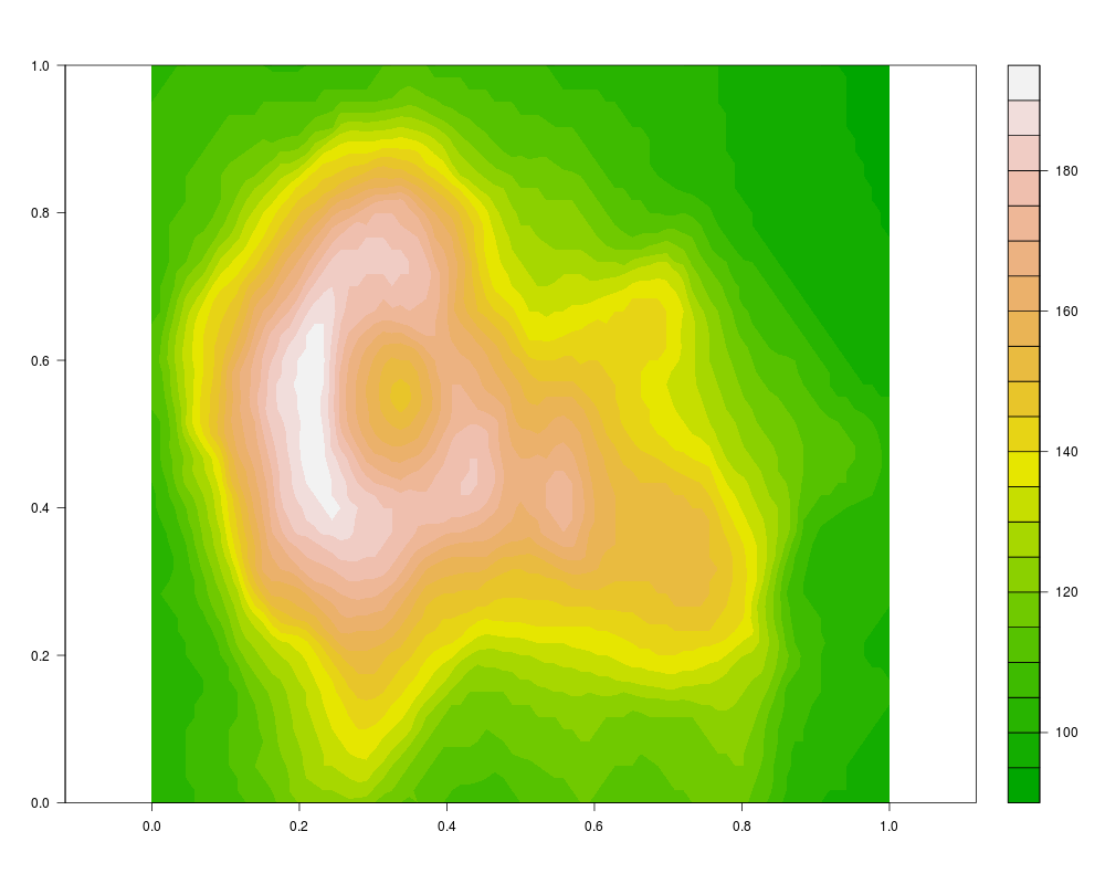
require(grDevices) # for colours
filled.contour(volcano, color = terrain.colors, asp = 1) # simple
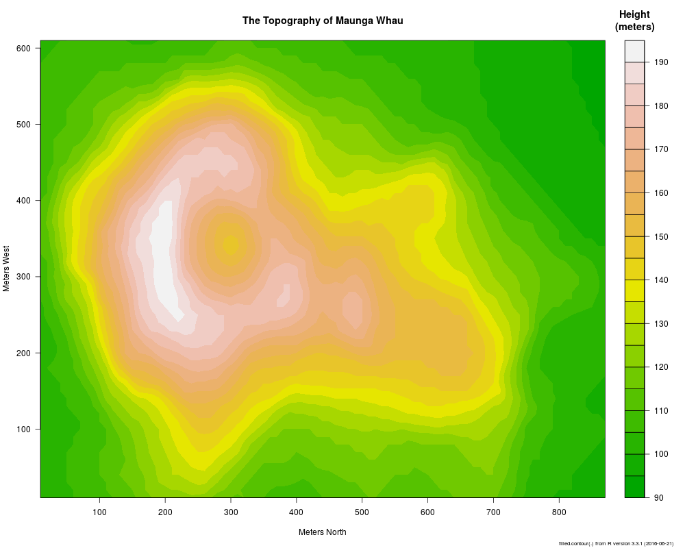
x <- 10*1:nrow(volcano)
y <- 10*1:ncol(volcano)
filled.contour(x, y, volcano, color = terrain.colors,
plot.title = title(main = "The Topography of Maunga Whau",
xlab = "Meters North", ylab = "Meters West"),
plot.axes = { axis(1, seq(100, 800, by = 100))
axis(2, seq(100, 600, by = 100)) },
key.title = title(main = "Height\n(meters)"),
key.axes = axis(4, seq(90, 190, by = 10))) # maybe also asp = 1
mtext(paste("filled.contour(.) from", R.version.string),
side = 1, line = 4, adj = 1, cex = .66)
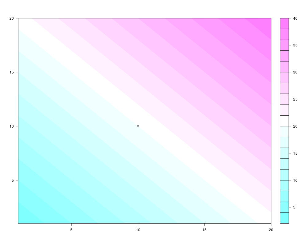
# Annotating a filled contour plot
a <- expand.grid(1:20, 1:20)
b <- matrix(a[,1] + a[,2], 20)
filled.contour(x = 1:20, y = 1:20, z = b,
plot.axes = { axis(1); axis(2); points(10, 10) })
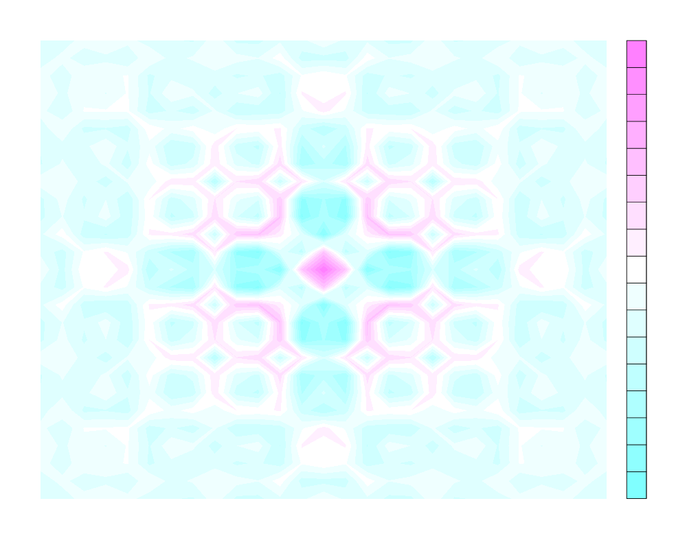
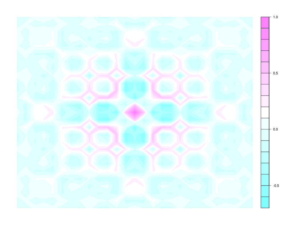
## Persian Rug Art:
x <- y <- seq(-4*pi, 4*pi, len = 27)
r <- sqrt(outer(x^2, y^2, "+"))
filled.contour(cos(r^2)*exp(-r/(2*pi)), axes = FALSE)
## rather, the key *should* be labeled:
filled.contour(cos(r^2)*exp(-r/(2*pi)), frame.plot = FALSE,
plot.axes = {})
Results
R version 3.3.1 (2016-06-21) -- "Bug in Your Hair"
Copyright (C) 2016 The R Foundation for Statistical Computing
Platform: x86_64-pc-linux-gnu (64-bit)

R is free software and comes with ABSOLUTELY NO WARRANTY.
You are welcome to redistribute it under certain conditions.
Type 'license()' or 'licence()' for distribution details.

R is a collaborative project with many contributors.
Type 'contributors()' for more information and
'citation()' on how to cite R or R packages in publications.

Type 'demo()' for some demos, 'help()' for on-line help, or
'help.start()' for an HTML browser interface to help.
Type 'q()' to quit R.

> library(graphics)
> png(filename="/home/ddbj/snapshot/RGM3/R_rel/result/graphics/filled.contour.Rd_%03d_medium.png", width=480, height=480)
> ### Name: filled.contour
> ### Title: Level (Contour) Plots
> ### Aliases: filled.contour .filled.contour
> ### Keywords: hplot aplot
>
> ### ** Examples
>
> require(grDevices) # for colours
> filled.contour(volcano, color = terrain.colors, asp = 1) # simple
>
> x <- 10*1:nrow(volcano)
> y <- 10*1:ncol(volcano)
> filled.contour(x, y, volcano, color = terrain.colors,
+     plot.title = title(main = "The Topography of Maunga Whau",
+     xlab = "Meters North", ylab = "Meters West"),
+     plot.axes = { axis(1, seq(100, 800, by = 100))
+                   axis(2, seq(100, 600, by = 100)) },
+     key.title = title(main = "Height\n(meters)"),
+     key.axes = axis(4, seq(90, 190, by = 10)))  # maybe also asp = 1
> mtext(paste("filled.contour(.) from", R.version.string),
+       side = 1, line = 4, adj = 1, cex = .66)
>
> # Annotating a filled contour plot
> a <- expand.grid(1:20, 1:20)
> b <- matrix(a[,1] + a[,2], 20)
> filled.contour(x = 1:20, y = 1:20, z = b,
+                plot.axes = { axis(1); axis(2); points(10, 10) })
>
> ## Persian Rug Art:
> x <- y <- seq(-4*pi, 4*pi, len = 27)
> r <- sqrt(outer(x^2, y^2, "+"))
> filled.contour(cos(r^2)*exp(-r/(2*pi)), axes = FALSE)
> ## rather, the key *should* be labeled:
> filled.contour(cos(r^2)*exp(-r/(2*pi)), frame.plot = FALSE,
+                plot.axes = {})
>
>
>
>
>
> dev.off()
null device
          1
>
|