Supported by Dr. Osamu Ogasawara and  . . |
|
Last data update: 2014.03.03 |
Differential NetworkDescriptionDifferential Network Usage
diffnet_multisplit(x1, x2, b.splits = 50, frac.split = 1/2,
  screen.meth = "screen_bic.glasso", include.mean = FALSE,
  gamma.min = 0.05, compute.evals = "est2.my.ev3",
  algorithm.mleggm = "glasso_rho0", method.compquadform = "imhof",
  acc = 1e-04, epsabs = 1e-10, epsrel = 1e-10, show.warn = FALSE,
  save.mle = FALSE, verbose = TRUE, mc.flag = FALSE, mc.set.seed = TRUE,
  mc.preschedule = TRUE, mc.cores = getOption("mc.cores", 2L), ...)
Arguments
DetailsRemark: * If include.mean=FALSE, then x1 and x2 have mean zero and DiffNet tests the hypothesis H0: Omega_1=Omega_2. You might need to center x1 and x2. * If include.mean=TRUE, then DiffNet tests the hypothesis H0: mu_1=mu_2 & Omega_1=Omega_2 * However, we recommend to set include.mean=FALSE and to test equality of the means separately. * You might also want to scale x1 and x2, if you are only interested in differences due to (partial) correlations. Valuelist consisting of
Author(s)n.stadler Examples
############################################################
##This example illustrates the use of Differential Network##
############################################################
##set seed
set.seed(1)
##sample size and number of nodes
n <- 40
p <- 10
##specifiy sparse inverse covariance matrices
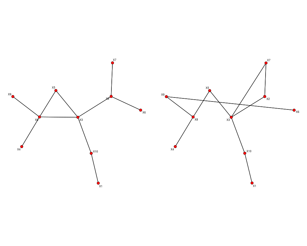
gen.net <- generate_2networks(p,graph='random',n.nz=rep(p,2),
n.nz.common=ceiling(p*0.8))
invcov1 <- gen.net[[1]]
invcov2 <- gen.net[[2]]
plot_2networks(invcov1,invcov2,label.pos=0,label.cex=0.7)
##get corresponding correlation matrices
cor1 <- cov2cor(solve(invcov1))
cor2 <- cov2cor(solve(invcov2))
##generate data under null hypothesis (both datasets have the same underlying
## network)
library('mvtnorm')
x1 <- rmvnorm(n,mean = rep(0,p), sigma = cor1)
x2 <- rmvnorm(n,mean = rep(0,p), sigma = cor1)
##run diffnet (under null hypothesis)
dn.null <- diffnet_multisplit(x1,x2,b.splits=1,verbose=FALSE)
dn.null$ss.pval#single-split p-value
##generate data under alternative hypothesis (datasets have different networks)
x1 <- rmvnorm(n,mean = rep(0,p), sigma = cor1)
x2 <- rmvnorm(n,mean = rep(0,p), sigma = cor2)
##run diffnet (under alternative hypothesis)
dn.altn <- diffnet_multisplit(x1,x2,b.splits=1,verbose=FALSE)
dn.altn$ss.pval#single-split p-value
dn.altn$medagg.pval#median aggregated p-value
##typically we would choose a larger number of splits
# dn.altn <- diffnet_multisplit(x1,x2,b.splits=10,verbose=FALSE)
# dn.altn$ms.pval#multi-split p-values
# dn.altn$medagg.pval#median aggregated p-value
# plot(dn.altn)#histogram of single-split p-values
Results
R version 3.3.1 (2016-06-21) -- "Bug in Your Hair"
Copyright (C) 2016 The R Foundation for Statistical Computing
Platform: x86_64-pc-linux-gnu (64-bit)

R is free software and comes with ABSOLUTELY NO WARRANTY.
You are welcome to redistribute it under certain conditions.
Type 'license()' or 'licence()' for distribution details.

R is a collaborative project with many contributors.
Type 'contributors()' for more information and
'citation()' on how to cite R or R packages in publications.

Type 'demo()' for some demos, 'help()' for on-line help, or
'help.start()' for an HTML browser interface to help.
Type 'q()' to quit R.

> library(nethet)
> png(filename="/home/ddbj/snapshot/RGM3/R_BC/result/nethet/diffnet_multisplit.Rd_%03d_medium.png", width=480, height=480)
> ### Name: diffnet_multisplit
> ### Title: Differential Network
> ### Aliases: diffnet_multisplit
>
> ### ** Examples
>
>
> ############################################################
> ##This example illustrates the use of Differential Network##
> ############################################################
>
>
> ##set seed
> set.seed(1)
>
> ##sample size and number of nodes
> n <- 40
> p <- 10
>
> ##specifiy sparse inverse covariance matrices
> gen.net <- generate_2networks(p,graph='random',n.nz=rep(p,2),
+                               n.nz.common=ceiling(p*0.8))
> invcov1 <- gen.net[[1]]
> invcov2 <- gen.net[[2]]
> plot_2networks(invcov1,invcov2,label.pos=0,label.cex=0.7)
>
> ##get corresponding correlation matrices
> cor1 <- cov2cor(solve(invcov1))
> cor2 <- cov2cor(solve(invcov2))
>
> ##generate data under null hypothesis (both datasets have the same underlying
> ## network)
> library('mvtnorm')
> x1 <- rmvnorm(n,mean = rep(0,p), sigma = cor1)
> x2 <- rmvnorm(n,mean = rep(0,p), sigma = cor1)
>
> ##run diffnet (under null hypothesis)
> dn.null <- diffnet_multisplit(x1,x2,b.splits=1,verbose=FALSE)
> dn.null$ss.pval#single-split p-value
[1] 0.9998887
>
> ##generate data under alternative hypothesis (datasets have different networks)
> x1 <- rmvnorm(n,mean = rep(0,p), sigma = cor1)
> x2 <- rmvnorm(n,mean = rep(0,p), sigma = cor2)
>
> ##run diffnet (under alternative hypothesis)
> dn.altn <- diffnet_multisplit(x1,x2,b.splits=1,verbose=FALSE)
> dn.altn$ss.pval#single-split p-value
[1] 0.0009634804
> dn.altn$medagg.pval#median aggregated p-value
[1] 0.0009634804
>
> ##typically we would choose a larger number of splits
> # dn.altn <- diffnet_multisplit(x1,x2,b.splits=10,verbose=FALSE)
> # dn.altn$ms.pval#multi-split p-values
> # dn.altn$medagg.pval#median aggregated p-value
> # plot(dn.altn)#histogram of single-split p-values
>
>
>
>
>
> dev.off()
null device
          1
>
|