Expression matrix for condition 1 (mean zero is required).
x2
Expression matrix for condition 2 (mean zero is required).
b.splits
Number of random data splits (default=50).
gene.sets
List of gene-sets.
gene.names
Gene names. Each column in x1 (and x2) corresponds
to a gene.
gs.names
Gene-set names (default=NULL).
method.p.adjust
Method for p-value adjustment (default='fdr').
order.adj.agg
Order of aggregation and adjustment of p-values.
Options: 'agg-adj' (default), 'adj-agg'.
mc.flag
If TRUE use parallel execution for each b.splits via function
mclapply of package parallel.
mc.set.seed
See mclapply. Default=TRUE
mc.preschedule
See mclapply. Default=TRUE
mc.cores
Number of cores to use in parallel execution. Defaults to
mc.cores option if set, or 2 otherwise.
verbose
If TRUE, show output progess.
...
Other arguments (see diffnet_singlesplit).
Details
Computation can be parallelized over many data splits.
Value
List consisting of
medagg.pval
Median aggregated p-values
meinshagg.pval
Meinshausen aggregated p-values
pval
matrix of p-values before correction and adjustement, dim(pval)=(number of gene-sets)x(number of splits)
teststatmed
median aggregated test-statistic
teststatmed.bic
median aggregated bic-corrected test-statistic
teststatmed.aic
median aggregated aic-corrected test-statistic
teststat
matrix of test-statistics, dim(teststat)=(number of gene-sets)x(number of splits)
rel.edgeinter
normalized intersection of edges in condition 1 and 2
df1
degrees of freedom of GGM obtained from condition 1
df2
degrees of freedom of GGM obtained from condition 2
df12
degrees of freedom of GGM obtained from pooled data (condition 1 and 2)
Author(s)
n.stadler
Examples
#######################################################
##This example illustrates the use of GGMGSA ##
#######################################################
## Generate networks
set.seed(1)
p <- 9#network with p nodes
n <- 40
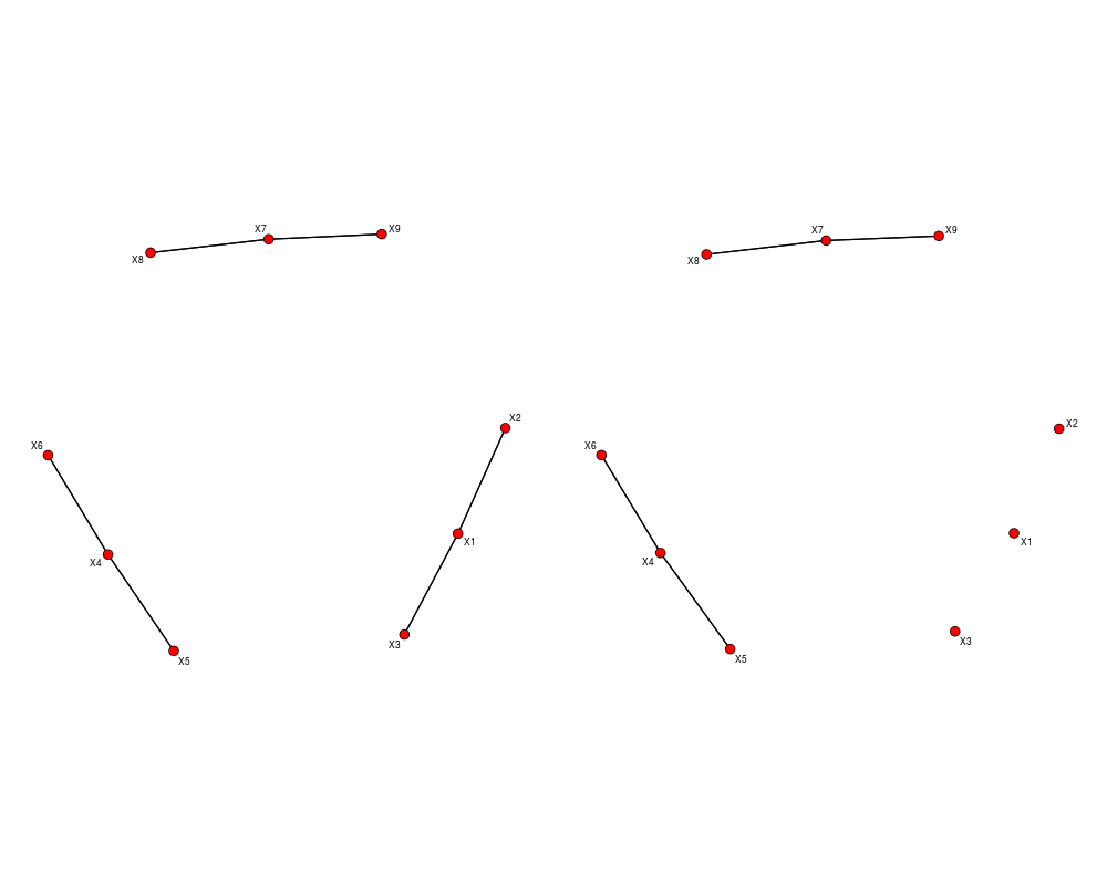
hub.net <- generate_2networks(p,graph='hub',n.hub=3,n.hub.diff=1)#generate hub networks
invcov1 <- hub.net[[1]]
invcov2 <- hub.net[[2]]
plot_2networks(invcov1,invcov2,label.pos=0,label.cex=0.7)
## Generate data
library('mvtnorm')
x1 <- rmvnorm(n,mean = rep(0,p), sigma = cov2cor(solve(invcov1)))
x2 <- rmvnorm(n,mean = rep(0,p), sigma = cov2cor(solve(invcov2)))
## Run DiffNet
# fit.dn <- diffnet_multisplit(x1,x2,b.splits=2,verbose=FALSE)
# fit.dn$medagg.pval
## Identify hubs with 'gene-sets'
gene.names <- paste('G',1:p,sep='')
gsets <- split(gene.names,rep(1:3,each=3))
## Run GGM-GSA
fit.ggmgsa <- ggmgsa_multisplit(x1,x2,b.splits=2,gsets,gene.names,verbose=FALSE)
summary(fit.ggmgsa)
fit.ggmgsa$medagg.pval#median aggregated p-values
p.adjust(apply(fit.ggmgsa$pval,1,median),method='fdr')#or: first median aggregation,
#second fdr-correction
Results
R version 3.3.1 (2016-06-21) -- "Bug in Your Hair"
Copyright (C) 2016 The R Foundation for Statistical Computing
Platform: x86_64-pc-linux-gnu (64-bit)

R is free software and comes with ABSOLUTELY NO WARRANTY.
You are welcome to redistribute it under certain conditions.
Type 'license()' or 'licence()' for distribution details.

R is a collaborative project with many contributors.
Type 'contributors()' for more information and
'citation()' on how to cite R or R packages in publications.

Type 'demo()' for some demos, 'help()' for on-line help, or
'help.start()' for an HTML browser interface to help.
Type 'q()' to quit R.

> library(nethet)
> png(filename="/home/ddbj/snapshot/RGM3/R_BC/result/nethet/ggmgsa_multisplit.Rd_%03d_medium.png", width=480, height=480)
> ### Name: ggmgsa_multisplit
> ### Title: Multi-split GGMGSA (parallelized computation)
> ### Aliases: ggmgsa_multisplit
>
> ### ** Examples
>
> #######################################################
> ##This example illustrates the use of GGMGSA         ##
> #######################################################
>
>
> ## Generate networks
> set.seed(1)
> p <- 9#network with p nodes
> n <- 40
> hub.net <- generate_2networks(p,graph='hub',n.hub=3,n.hub.diff=1)#generate hub networks
> invcov1 <- hub.net[[1]]
> invcov2 <- hub.net[[2]]
> plot_2networks(invcov1,invcov2,label.pos=0,label.cex=0.7)
>
> ## Generate data
> library('mvtnorm')
> x1 <- rmvnorm(n,mean = rep(0,p), sigma = cov2cor(solve(invcov1)))
> x2 <- rmvnorm(n,mean = rep(0,p), sigma = cov2cor(solve(invcov2)))
>
> ## Run DiffNet
> # fit.dn <- diffnet_multisplit(x1,x2,b.splits=2,verbose=FALSE)
> # fit.dn$medagg.pval
>
> ## Identify hubs with 'gene-sets'
> gene.names <- paste('G',1:p,sep='')
> gsets <- split(gene.names,rep(1:3,each=3))
>
> ## Run GGM-GSA
> fit.ggmgsa <- ggmgsa_multisplit(x1,x2,b.splits=2,gsets,gene.names,verbose=FALSE)
> summary(fit.ggmgsa)
    medagg.pval meinshagg.pval
gs1 0.001245657    0.005918268
gs2 0.414208743    1.000000000
gs3 0.414208743    1.000000000
> fit.ggmgsa$medagg.pval#median aggregated p-values
[1] 0.001245657 0.414208743 0.414208743
> p.adjust(apply(fit.ggmgsa$pval,1,median),method='fdr')#or: first median aggregation,
[1] 0.001245657 0.414208743 0.414208743
>                                                       #second fdr-correction
>
>
>
>
>
>
>
>
>
>
>
> dev.off()
null device
          1
>
 .
.