Number of mixture components. If n.comp is a vector,
mixglasso will estimate a model for each number of mixture components,
and return a list of models, as well as their BIC and MMDL scores and the index of the
best model according to each score.
Determines form of penalty: glasso.parcor (default) to penalise the
partial correlation matrix, glasso.invcov to penalise the inverse covariance
matrix (this corresponds to classical graphical lasso), glasso.invcor to
penalise the inverse correlation matrix.
init
Initialization. Method used for initialization
init='cl.init','r.means','random','kmeans','kmeans.hc','hc'. Default='kmeans'
my.cl
Initial cluster assignments;
need to be provided if init='cl.init' (otherwise this param is ignored). Default=NULL
modelname.hc
Model class used in hc. Default="VVV"
nstart.kmeans
Number of random starts in kmeans; default=1
iter.max.kmeans
Maximal number of iteration in kmeans; default=10
term
Termination criterion of EM algorithm. Default=10^-3
min.compsize
Stop EM if any(compsize)<min.compsize; Default=5
save.allfits
If TRUE, save output of mixglasso for all k's.
filename
If save.allfits is TRUE, output of mixglasso will be
saved as paste(filename, _fit.mixgl_k.rda, sep='').
mc.flag
If TRUE use parallel execution for each n.comp via function
mclapply of package parallel.
mc.set.seed
See mclapply. Default=FALSE
mc.preschedule
See mclapply. Default=FALSE
mc.cores
Number of cores to use in parallel execution. Defaults to
mc.cores option if set, or 2 otherwise.
...
Other arguments. See mixglasso_init
Details
Runs mixture of graphical lasso network clustering with one or several
numbers of mixture components.
Value
A list with elements:
models
List with each element i containing an S3 object of class
'nethetclustering' that contains the result of fitting the mixture
graphical lasso model with n.comps[i] components. See the documentation of
mixglasso_ncomp_fixed for the description of this object.
bic
BIC for all fits.
mmdl
Minimum description length score for all fits.
comp
Component assignments for all fits.
bix.opt
Index of model with optimal BIC score.
mmdl.opt
Index of model with optimal MMDL score.
Author(s)
n.stadler
Examples
###########################################
##This an example of how to use MixGLasso##
###########################################
##generate data
set.seed(1)
n <- 1000
n.comp <- 3
p <- 10
# Create different mean vectors
Mu <- matrix(0,p,n.comp)
nonzero.mean <- split(sample(1:p),rep(1:n.comp,length=p))
for(k in 1:n.comp){
Mu[nonzero.mean[[k]],k] <- -2/sqrt(ceiling(p/n.comp))
}
sim <- sim_mix_networks(n, p, n.comp, Mu=Mu)
##run mixglasso
set.seed(1)
fit1 <- mixglasso(sim$data,n.comp=1:6)
fit1$bic
set.seed(1)
fit2 <- mixglasso(sim$data,n.comp=6)
fit2$bic
set.seed(1)
fit3 <- mixglasso(sim$data,n.comp=1:6,lambda=0)
set.seed(1)
fit4 <- mixglasso(sim$data,n.comp=1:6,lambda=Inf)
#set.seed(1)
#fit5 <- bwprun_mixglasso(sim$data,n.comp=1,n.comp.max=5,selection.crit='bic')
#plot(fit5$selcrit,ylab='bic',xlab='Num.Comps',type='b')
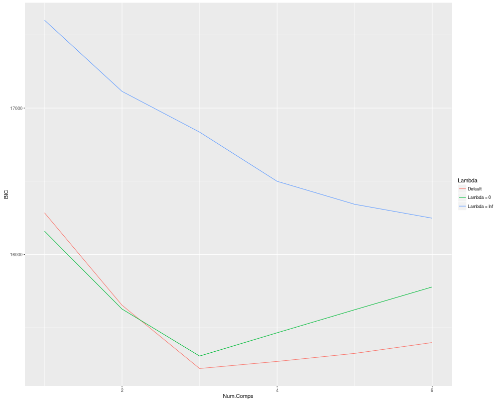
##compare bic
library('ggplot2')
plotting.frame <- data.frame(BIC= c(fit1$bic, fit3$bic, fit4$bic),
Num.Comps=rep(1:6, 3), Lambda=rep(
c('Default',
'Lambda = 0',
'Lambda = Inf'),
each=6))
p <- ggplot(plotting.frame) +
geom_line(aes(x=Num.Comps, y=BIC, colour=Lambda))
print(p)
Results
R version 3.3.1 (2016-06-21) -- "Bug in Your Hair"
Copyright (C) 2016 The R Foundation for Statistical Computing
Platform: x86_64-pc-linux-gnu (64-bit)

R is free software and comes with ABSOLUTELY NO WARRANTY.
You are welcome to redistribute it under certain conditions.
Type 'license()' or 'licence()' for distribution details.

R is a collaborative project with many contributors.
Type 'contributors()' for more information and
'citation()' on how to cite R or R packages in publications.

Type 'demo()' for some demos, 'help()' for on-line help, or
'help.start()' for an HTML browser interface to help.
Type 'q()' to quit R.

> library(nethet)
> png(filename="/home/ddbj/snapshot/RGM3/R_BC/result/nethet/mixglasso.Rd_%03d_medium.png", width=480, height=480)
> ### Name: mixglasso
> ### Title: mixglasso
> ### Aliases: mixglasso
>
> ### ** Examples
>
>
>
> ###########################################
> ##This an example of how to use MixGLasso##
> ###########################################
>
> ##generate data
> set.seed(1)
> n <- 1000
> n.comp <- 3
> p <- 10
>
> # Create different mean vectors
> Mu <- matrix(0,p,n.comp)
>
> nonzero.mean <- split(sample(1:p),rep(1:n.comp,length=p))
> for(k in 1:n.comp){
+   Mu[nonzero.mean[[k]],k] <- -2/sqrt(ceiling(p/n.comp))
+ }
>
> sim <- sim_mix_networks(n, p, n.comp, Mu=Mu)
>
> ##run mixglasso
> set.seed(1)
> fit1 <-  mixglasso(sim$data,n.comp=1:6)
> fit1$bic
[1] 16284.46 15653.10 15220.72 15269.09 15324.06 15398.23
> set.seed(1)
> fit2 <-  mixglasso(sim$data,n.comp=6)
> fit2$bic
[1] 15398.23
> set.seed(1)
> fit3 <-  mixglasso(sim$data,n.comp=1:6,lambda=0)
> set.seed(1)
> fit4 <-  mixglasso(sim$data,n.comp=1:6,lambda=Inf)
> #set.seed(1)
> #fit5 <-  bwprun_mixglasso(sim$data,n.comp=1,n.comp.max=5,selection.crit='bic')
> #plot(fit5$selcrit,ylab='bic',xlab='Num.Comps',type='b')
>
> ##compare bic
> library('ggplot2')
> plotting.frame <- data.frame(BIC= c(fit1$bic, fit3$bic, fit4$bic),
+ 														 Num.Comps=rep(1:6, 3), Lambda=rep(
+ 														 	                        c('Default',
+ 														 													  'Lambda = 0',
+ 														 														'Lambda = Inf'),
+ 														 													each=6))
>
> p <- ggplot(plotting.frame) +
+ 	geom_line(aes(x=Num.Comps, y=BIC, colour=Lambda))
>
> print(p)
>
>
>
>
>
> dev.off()
null device
          1
>
 .
.