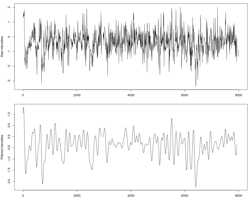
Clean noise and smoothing for genomic data using Fourier-analysis

Description

Remove noise from genomic data smoothing and cleaning the observed signal. This function doesn't alter the shape or the values of the signal as much as the traditional method of sliding window average does, providing a great correlation within the original and filtered data (>0.99).

Usage

## S4 method for signature 'SimpleRleList'
filterFFT(data, pcKeepComp="auto", showPowerSpec=FALSE, useOptim=TRUE, mc.cores=1, ...)
## S4 method for signature 'list'
filterFFT(data, pcKeepComp="auto", showPowerSpec=FALSE, useOptim=TRUE, mc.cores=1, ...)
## S4 method for signature 'Rle'
filterFFT(data, pcKeepComp="auto", showPowerSpec=FALSE, useOptim=TRUE, ...)
## S4 method for signature 'numeric'
filterFFT(data, pcKeepComp="auto", showPowerSpec=FALSE, useOptim=TRUE, ...)

Arguments

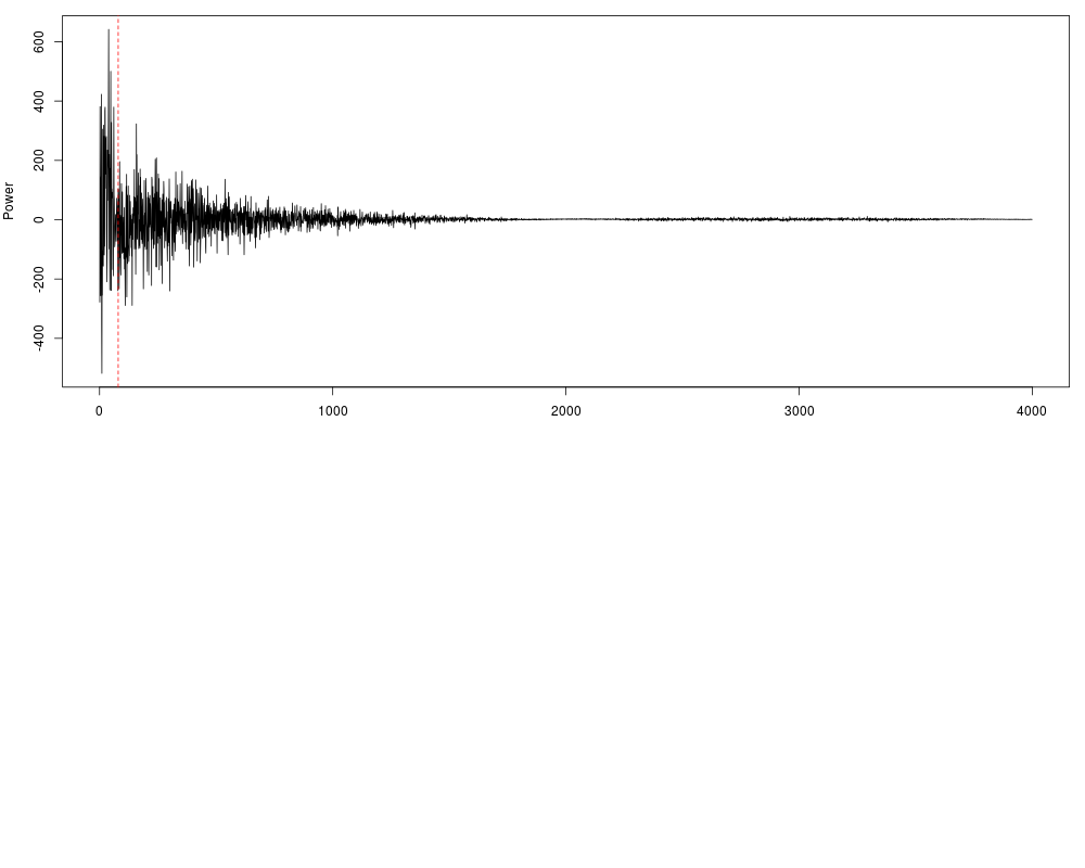
Details

Fourier-analysis principal components selection is widely used in signal processing theory for an unbiased cleaning of a signal over the time.

Other procedures, as the traditional sliding window average, can change too much the shape of the results in function of the size of the window, and moreover they don't only smooth the noise without removing it.

With a Fourier Transform of the original signal, the input signal is descomposed in diferent wavelets and described as a combination of them. Long frequencies can be explained as a function of two ore more periodical shorter frequecies. This is the reason why long, unperiodic sequences are usually identified as noise, and therefore is desireable to remove them from the signal we have to process.

This procedure here is applied to genomic data, providing a novel method to obtain perfectly clean values wich allow an efficient detection of the peaks which can be used for a direct nucleosome position recognition.

This function select a certain number of components in the original power spectrum (the result of the Fast Fourier Transform which can be seen with showPowerSpec=TRUE) and sets the rest of them to 0 (component knock-out).

The amout of components to keep (given as a percentage of the input lenght) can be set by the pcKeepComp. This will select the first components of the signal, knock-outing the rest. If this value is close to 1, more components will be selected and then more noise will be allowed in the output. For an effective filtering which removes the noise keeping almost all relevant peaks, a value between 0.01 and 0.05 is usually sufficient. Lower values can cause merging of adjacent minor peaks.

This library also allows the automatic detection of a fitted value for pcKeepComp. By default, if uses the pcKeepCompDetect function, which looks which is the minimum percentage of components than can reproduce the original signal with a corelation between the filtered and the original one of 0.99. See the help page of pcKeepCompDetect for further details and reference of available parameters.

One of the most powerful features of nucleR is the efficient implementation of the FFT to genomic data. This is achived trought few tweaks that allow an optimum performance of the Fourier Transform. This includes a by-range filtering, an automatic detection of uncovered regions, windowed execution of the filter and padding of the data till nearest power of 2 (this ensures an optimum case for FFT due the high factorization of components). Internal testing showed up that in specific datasets, these optimizations lead to a dramatic improvement of many orders of magnitude (from 3 days to few seconds) while keeping the correlation between the native fft call and our filterFFT higher than 0.99. So, the use of these optimizations is highly recomended.

If for some reason you want to apply the function without any kind of optimizations you can specify the parameter useOptim=FALSE to bypass them and get the pure knockout inverse from native FFT call. All other parameters can be still applyied in this case.

Value

Numeric vector with cleaned/smoothed values

Author(s)

Oscar Flores oflores@mmb.pcb.ub.es, David Rosell david.rossell@irbbarcelona.org

References

Smith, Steven W. (1999), The Scientist and Engineer's Guide to Digital Signal Processing (Second ed.), San Diego, Calif.: California Technical Publishing, ISBN 0-9660176-3-3 (availabe online: http://www.dspguide.com/pdfbook.htm)

Examples

	#Load example data, raw hybridization values for Tiling Array
	raw_data = get(data(nucleosome_tiling))
	
	#Filter data
	fft_data = filterFFT(raw_data, pcKeepComp=0.01)

	#See both profiles
	par(mfrow=c(2,1), mar=c(3, 4, 1, 1))
	plot(raw_data, type="l", xlab="position", ylab="Raw intensities")
	plot(fft_data, type="l", xlab="position", ylab="Filtered intensities")

	#The power spectrum shows a visual representation of the components
	fft_data = filterFFT(raw_data, pcKeepComp=0.01, showPowerSpec=TRUE)

Results

R version 3.3.1 (2016-06-21) -- "Bug in Your Hair"
Copyright (C) 2016 The R Foundation for Statistical Computing
Platform: x86_64-pc-linux-gnu (64-bit)

R is free software and comes with ABSOLUTELY NO WARRANTY.
You are welcome to redistribute it under certain conditions.
Type 'license()' or 'licence()' for distribution details.

R is a collaborative project with many contributors.
Type 'contributors()' for more information and
'citation()' on how to cite R or R packages in publications.

Type 'demo()' for some demos, 'help()' for on-line help, or
'help.start()' for an HTML browser interface to help.
Type 'q()' to quit R.

> library(nucleR)
Loading required package: ShortRead
Loading required package: BiocGenerics
Loading required package: parallel

Attaching package: 'BiocGenerics'

The following objects are masked from 'package:parallel':

    clusterApply, clusterApplyLB, clusterCall, clusterEvalQ,
    clusterExport, clusterMap, parApply, parCapply, parLapply,
    parLapplyLB, parRapply, parSapply, parSapplyLB

The following objects are masked from 'package:stats':

    IQR, mad, xtabs

The following objects are masked from 'package:base':

    Filter, Find, Map, Position, Reduce, anyDuplicated, append,
    as.data.frame, cbind, colnames, do.call, duplicated, eval, evalq,
    get, grep, grepl, intersect, is.unsorted, lapply, lengths, mapply,
    match, mget, order, paste, pmax, pmax.int, pmin, pmin.int, rank,
    rbind, rownames, sapply, setdiff, sort, table, tapply, union,
    unique, unsplit

Loading required package: BiocParallel
Loading required package: Biostrings
Loading required package: S4Vectors
Loading required package: stats4

Attaching package: 'S4Vectors'

The following objects are masked from 'package:base':

    colMeans, colSums, expand.grid, rowMeans, rowSums

Loading required package: IRanges
Loading required package: XVector
Loading required package: Rsamtools
Loading required package: GenomeInfoDb
Loading required package: GenomicRanges
Loading required package: GenomicAlignments
Loading required package: SummarizedExperiment
Loading required package: Biobase
Welcome to Bioconductor

    Vignettes contain introductory material; view with
    'browseVignettes()'. To cite Bioconductor, see
    'citation("Biobase")', and for packages 'citation("pkgname")'.

> png(filename="/home/ddbj/snapshot/RGM3/R_BC/result/nucleR/filterFFT.Rd_%03d_medium.png", width=480, height=480)
> ### Name: filterFFT
> ### Title: Clean noise and smoothing for genomic data using
> ###   Fourier-analysis
> ### Aliases: filterFFT filterFFT,SimpleRleList-method filterFFT,Rle-method
> ###   filterFFT,list-method filterFFT,numeric-method
> ### Keywords: manip
> 
> ### ** Examples
> 
> 	#Load example data, raw hybridization values for Tiling Array
> 	raw_data = get(data(nucleosome_tiling))
> 	
> 	#Filter data
> 	fft_data = filterFFT(raw_data, pcKeepComp=0.01)
> 
> 	#See both profiles
> 	par(mfrow=c(2,1), mar=c(3, 4, 1, 1))
> 	plot(raw_data, type="l", xlab="position", ylab="Raw intensities")
> 	plot(fft_data, type="l", xlab="position", ylab="Filtered intensities")
> 
> 	#The power spectrum shows a visual representation of the components
> 	fft_data = filterFFT(raw_data, pcKeepComp=0.01, showPowerSpec=TRUE)
> 
> 
> 
> 
> 
> dev.off()
null device 
          1 
>