Nucleosome positioning package for R

Description

Nucleosome positioning from Tiling Arrays and High-Troughput Sequencing Experiments

Details

This package provides a convenient pipeline to process and analize nucleosome positioning experiments from High-Troughtput Sequencing or Tiling Arrays.

Despite it's use is intended to nucleosome experiments, it can be also useful for general ChIP experiments, such as ChIP-on-ChIP or ChIP-Seq.

See following example for a brief introduction to the available functions

Author(s)

Oscar Flores Ricard Illa

Maintainer: Ricard Illa <ricard.illa@irbbarcelona.org>

Examples

    #Load example dataset:
    # some NGS paired-end reads, mapped with Bowtie and processed with R
    # it is a RangedData object with the start/end coordinates for each read.
    reads = get(data(nucleosome_htseq))

    #Process the paired end reads, but discard those with length > 200
    preads_orig = processReads(reads, type="paired", fragmentLen=200)

    #Process the reads, but now trim each read to 40bp around the dyad
    preads_trim = processReads(reads, type="paired", fragmentLen=200, trim=40)

    #Calculate the coverage, directly in reads per million (r.p.m)
    cover_orig = coverage.rpm(preads_orig)
    cover_trim = coverage.rpm(preads_trim)

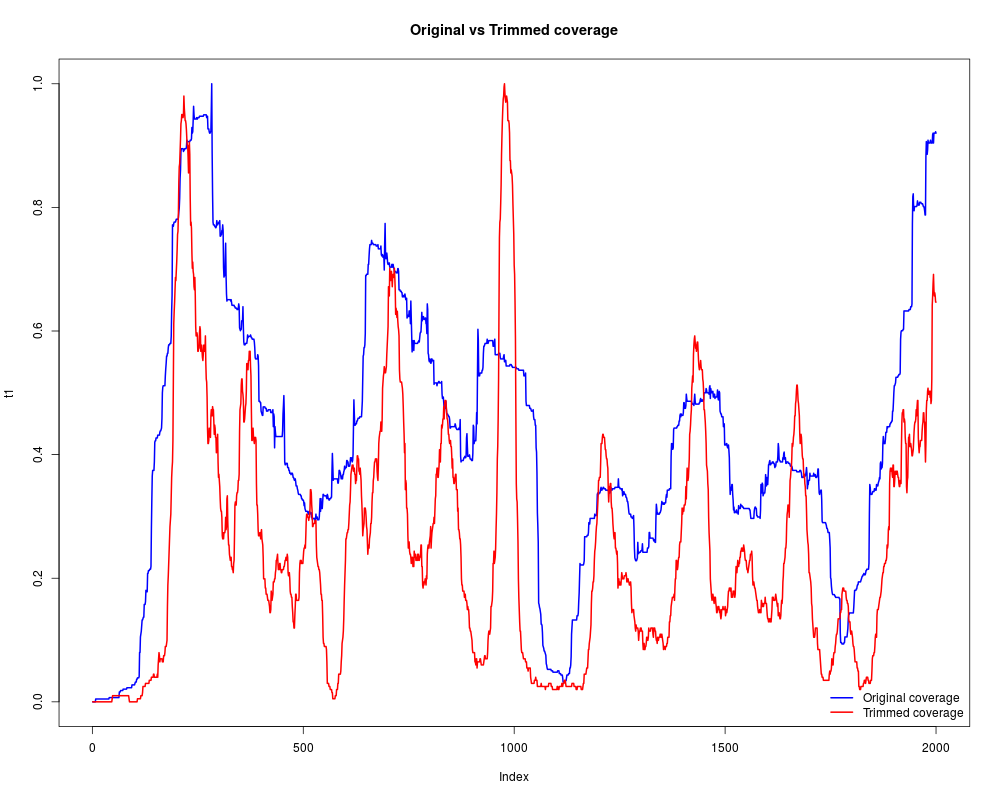
    #Compare both coverages, the dyad is much more clear in trimmed version
    t1 = as.vector(cover_orig[[1]])[1:2000]
    t2 = as.vector(cover_trim[[1]])[1:2000]
    t1 = (t1-min(t1))/max(t1-min(t1)) #Normalization
    t2 = (t2-min(t2))/max(t2-min(t2)) #Normalization
    plot(t1, type="l", lwd="2", col="blue", main="Original vs Trimmed coverage")
    lines(t2, lwd="2", col="red")
    legend("bottomright", c("Original coverage", "Trimmed coverage"), lwd=2, col=c("blue","red"), bty="n")

    #Let's try to call nucleosomes from the trimmed version
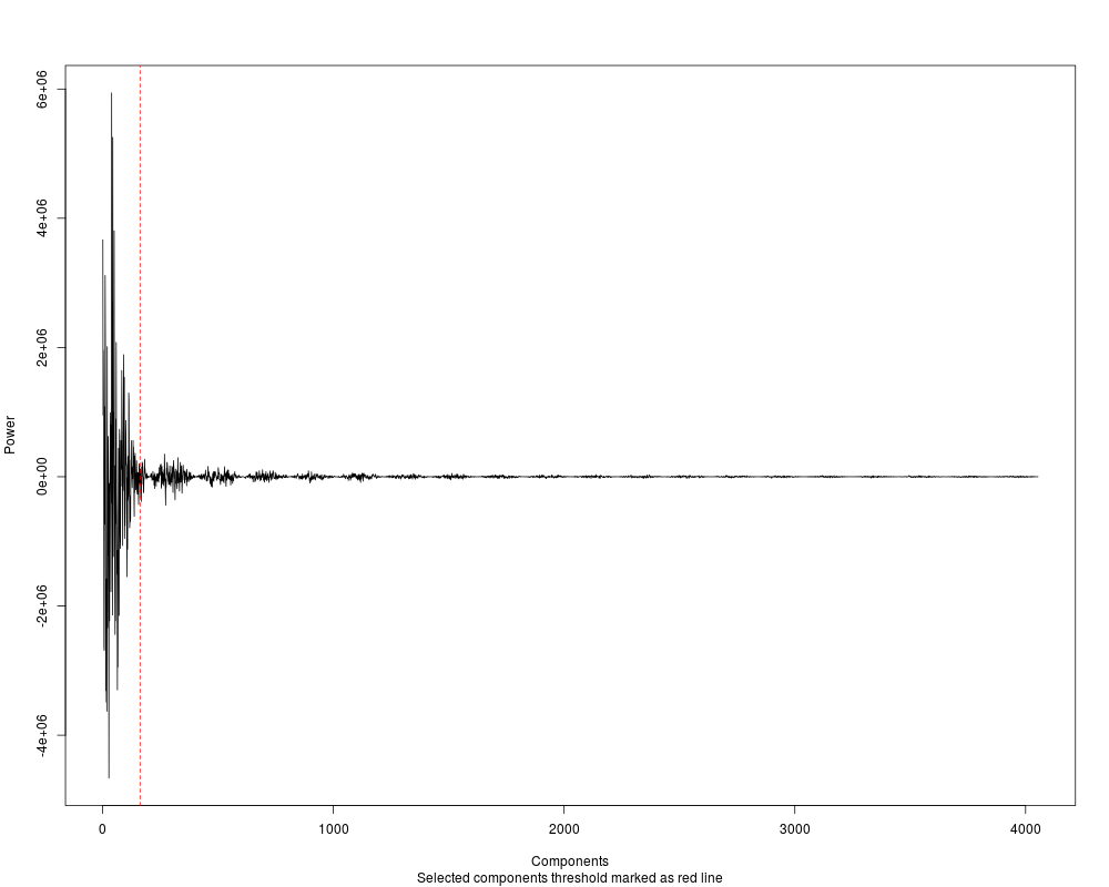
    #First of all, let's remove some noise with FFT
    #Power spectrum will be plotted, look how with a 2%
    #of the components we capture almost all the signal
    cover_clean = filterFFT(cover_trim, pcKeepComp=0.02, showPowerSpec=TRUE)

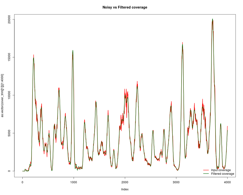
    #How clean is now?
    plot(as.vector(cover_trim[[1]])[1:4000], t="l", lwd=2, col="red", main="Noisy vs Filtered coverage")
    lines(cover_clean[[1]][1:4000], lwd=2, col="darkgreen")
    legend("bottomright", c("Input coverage", "Filtered coverage"), lwd=2, col=c("red","darkgreen"), bty="n")

    #And how similar? Let's see the correlation
    cor(cover_clean[[1]], as.vector(cover_trim[[1]]))

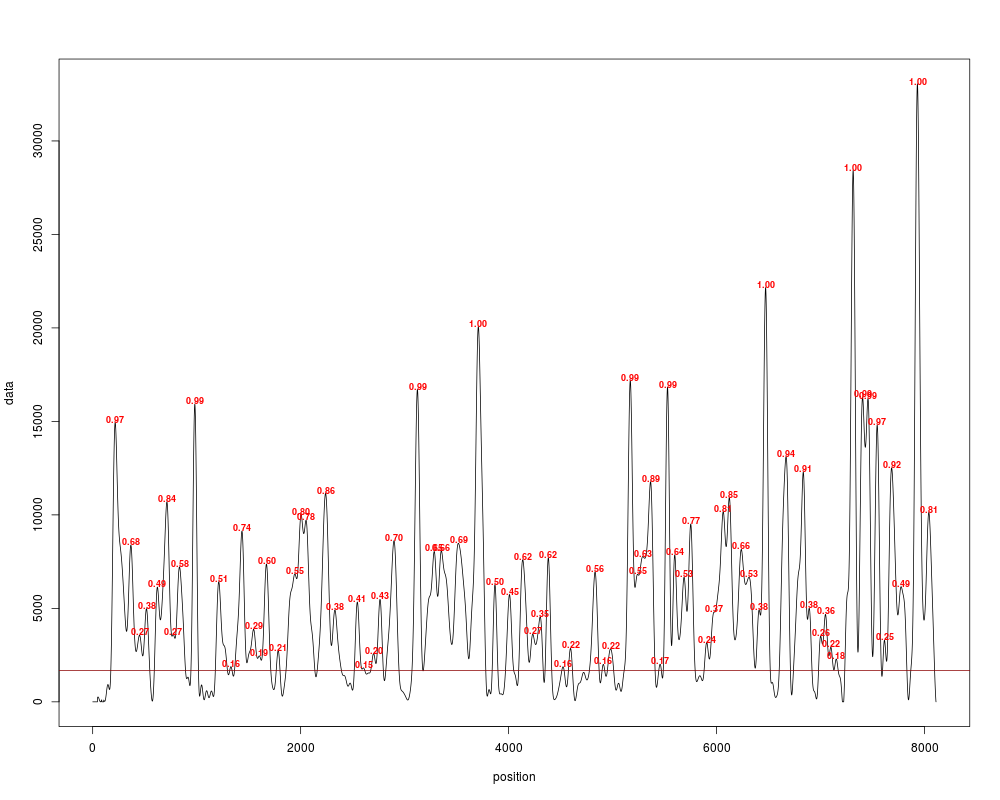
    #Now it's time to call for peaks, first just as points
    #See that the score is only a measure of the height of the peak
    peaks = peakDetection(cover_clean, threshold="25%", score=TRUE)
    plotPeaks(peaks[[1]], cover_clean[[1]], threshold="25%")

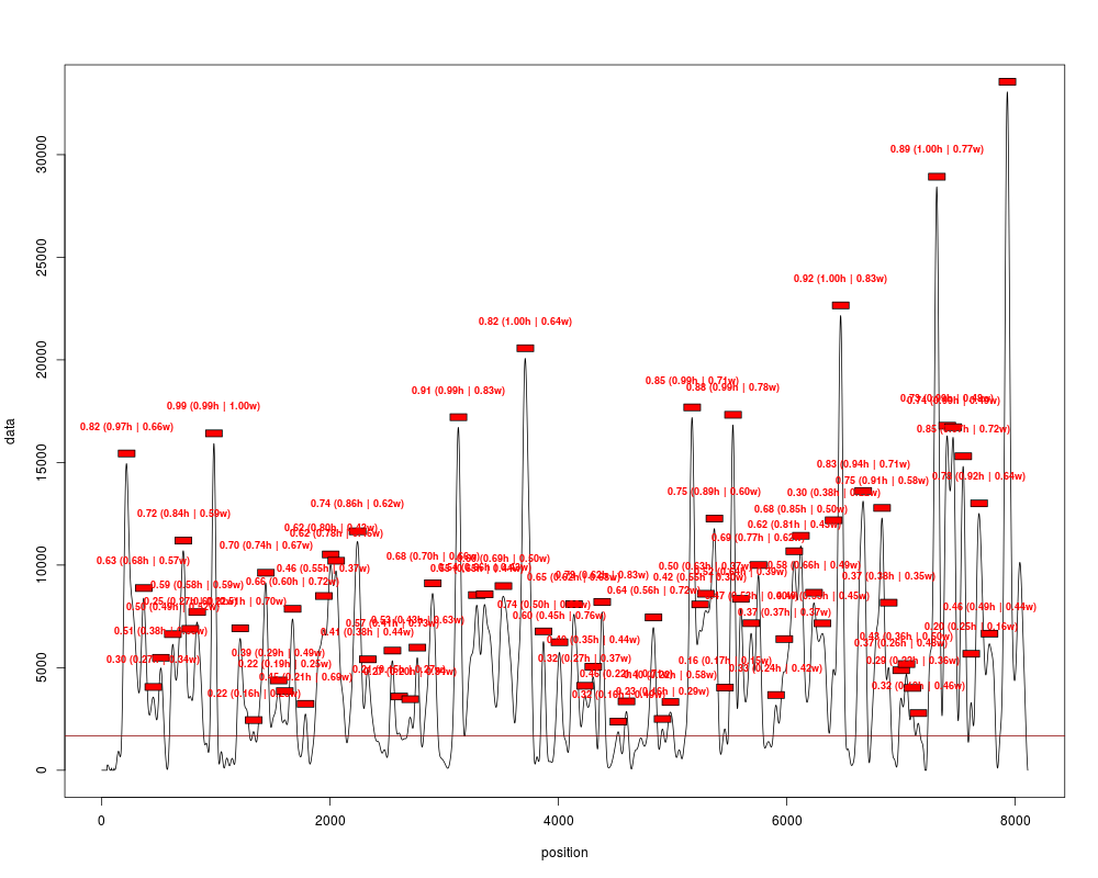
    #Do the same as previously, but now we will create the nucleosome calls:
    peaks = peakDetection(cover_clean, width=147, threshold="25%", score=TRUE)
    plotPeaks(peaks, cover_clean[[1]], threshold="25%")

    #This is all. From here, you can filter, merge or work with the nucleosome
    #calls using standard IRanges functions and R/Bioconductor manipulation

Results

R version 3.3.1 (2016-06-21) -- "Bug in Your Hair"
Copyright (C) 2016 The R Foundation for Statistical Computing
Platform: x86_64-pc-linux-gnu (64-bit)

R is free software and comes with ABSOLUTELY NO WARRANTY.
You are welcome to redistribute it under certain conditions.
Type 'license()' or 'licence()' for distribution details.

R is a collaborative project with many contributors.
Type 'contributors()' for more information and
'citation()' on how to cite R or R packages in publications.

Type 'demo()' for some demos, 'help()' for on-line help, or
'help.start()' for an HTML browser interface to help.
Type 'q()' to quit R.

> library(nucleR)
Loading required package: ShortRead
Loading required package: BiocGenerics
Loading required package: parallel

Attaching package: 'BiocGenerics'

The following objects are masked from 'package:parallel':

    clusterApply, clusterApplyLB, clusterCall, clusterEvalQ,
    clusterExport, clusterMap, parApply, parCapply, parLapply,
    parLapplyLB, parRapply, parSapply, parSapplyLB

The following objects are masked from 'package:stats':

    IQR, mad, xtabs

The following objects are masked from 'package:base':

    Filter, Find, Map, Position, Reduce, anyDuplicated, append,
    as.data.frame, cbind, colnames, do.call, duplicated, eval, evalq,
    get, grep, grepl, intersect, is.unsorted, lapply, lengths, mapply,
    match, mget, order, paste, pmax, pmax.int, pmin, pmin.int, rank,
    rbind, rownames, sapply, setdiff, sort, table, tapply, union,
    unique, unsplit

Loading required package: BiocParallel
Loading required package: Biostrings
Loading required package: S4Vectors
Loading required package: stats4

Attaching package: 'S4Vectors'

The following objects are masked from 'package:base':

    colMeans, colSums, expand.grid, rowMeans, rowSums

Loading required package: IRanges
Loading required package: XVector
Loading required package: Rsamtools
Loading required package: GenomeInfoDb
Loading required package: GenomicRanges
Loading required package: GenomicAlignments
Loading required package: SummarizedExperiment
Loading required package: Biobase
Welcome to Bioconductor

    Vignettes contain introductory material; view with
    'browseVignettes()'. To cite Bioconductor, see
    'citation("Biobase")', and for packages 'citation("pkgname")'.

> png(filename="/home/ddbj/snapshot/RGM3/R_BC/result/nucleR/nucleR-package.Rd_%03d_medium.png", width=480, height=480)
> ### Name: nucleR-package
> ### Title: Nucleosome positioning package for R
> ### Aliases: nucleR-package nucleR
> ### Keywords: package
> 
> ### ** Examples
> 
> 
>     #Load example dataset:
>     # some NGS paired-end reads, mapped with Bowtie and processed with R
>     # it is a RangedData object with the start/end coordinates for each read.
>     reads = get(data(nucleosome_htseq))
> 
>     #Process the paired end reads, but discard those with length > 200
>     preads_orig = processReads(reads, type="paired", fragmentLen=200)
> 
>     #Process the reads, but now trim each read to 40bp around the dyad
>     preads_trim = processReads(reads, type="paired", fragmentLen=200, trim=40)
> 
>     #Calculate the coverage, directly in reads per million (r.p.m)
>     cover_orig = coverage.rpm(preads_orig)
>     cover_trim = coverage.rpm(preads_trim)
> 
>     #Compare both coverages, the dyad is much more clear in trimmed version
>     t1 = as.vector(cover_orig[[1]])[1:2000]
>     t2 = as.vector(cover_trim[[1]])[1:2000]
>     t1 = (t1-min(t1))/max(t1-min(t1)) #Normalization
>     t2 = (t2-min(t2))/max(t2-min(t2)) #Normalization
>     plot(t1, type="l", lwd="2", col="blue", main="Original vs Trimmed coverage")
>     lines(t2, lwd="2", col="red")
>     legend("bottomright", c("Original coverage", "Trimmed coverage"), lwd=2, col=c("blue","red"), bty="n")
> 
>     #Let's try to call nucleosomes from the trimmed version
>     #First of all, let's remove some noise with FFT
>     #Power spectrum will be plotted, look how with a 2%
>     #of the components we capture almost all the signal
>     cover_clean = filterFFT(cover_trim, pcKeepComp=0.02, showPowerSpec=TRUE)
> 
>     #How clean is now?
>     plot(as.vector(cover_trim[[1]])[1:4000], t="l", lwd=2, col="red", main="Noisy vs Filtered coverage")
>     lines(cover_clean[[1]][1:4000], lwd=2, col="darkgreen")
>     legend("bottomright", c("Input coverage", "Filtered coverage"), lwd=2, col=c("red","darkgreen"), bty="n")
> 
>     #And how similar? Let's see the correlation
>     cor(cover_clean[[1]], as.vector(cover_trim[[1]]))
[1] 0.9937643
> 
>     #Now it's time to call for peaks, first just as points
>     #See that the score is only a measure of the height of the peak
>     peaks = peakDetection(cover_clean, threshold="25%", score=TRUE)
>     plotPeaks(peaks[[1]], cover_clean[[1]], threshold="25%")
> 
>     #Do the same as previously, but now we will create the nucleosome calls:
>     peaks = peakDetection(cover_clean, width=147, threshold="25%", score=TRUE)
>     plotPeaks(peaks, cover_clean[[1]], threshold="25%")
> 
>     #This is all. From here, you can filter, merge or work with the nucleosome
>     #calls using standard IRanges functions and R/Bioconductor manipulation
> 
> 
> 
> 
> 
> dev.off()
null device 
          1 
>