R Graphical Manual

Browse All

Last data update: 2014.03.03

R: Calculate Double Principle Coordinate Analysis (DPCoA) using...

DPCoA

R Documentation

Calculate Double Principle Coordinate Analysis (DPCoA) using phylogenetic distance

Description

Function uses abundance (otu_table-class) and phylogenetic (phylo) components of a phyloseq-class experiment-level object to perform a Double Principle Coordinate Analysis (DPCoA), relying heavily on the underlying (and more general) function, dpcoa. The distance object ultimately provided as the cophenetic/patristic (cophenetic.phylo) distance between the species.

Usage

DPCoA(physeq, correction = cailliez, scannf = FALSE, ...)

Arguments

`physeq`	(Required). A `phyloseq-class` object containing, at a minimum, abundance (`otu_table-class`) and phylogenetic (`phylo`) components. As a test, the accessors `otu_table` and `phy_tree` should return an object without error.
`correction`	(Optional). A function. The function must be able to take a non-Euclidean `dist`ance object, and return a new `dist`ance object that is Euclidean. If testing a distance object, try `is.euclid`. In most real-life, real-data applications, the phylogenetic tree will not provide a Euclidean distance matrix, and so a correction will be needed. Two recommended correction methods are `cailliez` and `lingoes`. The default is `cailliez`, but not for any particularly special reason. If the patristic distance matrix turns out to be Euclidian, no correction will be performed, regardless of the value of the `correction` argument.
`scannf`	(Optional). Logical. Default is `FALSE`. This is passed directly to `dpcoa`, and causes a barplot of eigenvalues to be created if `TRUE`. This is not included in `...` because the default for `dpcoa` is `TRUE`, although in many expected situations we would want to suppress creating the barplot.
`...`	Additional arguments passed to `dpcoa`.

Details

In most real-life, real-data applications, the phylogenetic tree will not provide a Euclidean distance matrix, and so a correction will be performed, if needed. See correction argument.

Value

A dpcoa-class object (see dpcoa).

Author(s)

Julia Fukuyama julia.fukuyama@gmail.com. Adapted for phyloseq by Paul J. McMurdie.

References

Pavoine, S., Dufour, A.B. and Chessel, D. (2004) From dissimilarities among species to dissimilarities among communities: a double principal coordinate analysis. Journal of Theoretical Biology, 228, 523-537.

Examples

# # # # # # Esophagus
data(esophagus)
eso.dpcoa <- DPCoA(esophagus)
eso.dpcoa
plot_ordination(esophagus, eso.dpcoa, "samples")
plot_ordination(esophagus, eso.dpcoa, "species")
plot_ordination(esophagus, eso.dpcoa, "biplot")
#
#
# # # # # # GlobalPatterns
data(GlobalPatterns)
# subset GP to top-150 taxa (to save computation time in example)
keepTaxa <- names(sort(taxa_sums(GlobalPatterns), TRUE)[1:150])
GP       <- prune_taxa(keepTaxa, GlobalPatterns)
# Perform DPCoA
GP.dpcoa <- DPCoA(GP)
plot_ordination(GP, GP.dpcoa, color="SampleType")

Results


R version 3.3.1 (2016-06-21) -- "Bug in Your Hair"
Copyright (C) 2016 The R Foundation for Statistical Computing
Platform: x86_64-pc-linux-gnu (64-bit)

R is free software and comes with ABSOLUTELY NO WARRANTY.
You are welcome to redistribute it under certain conditions.
Type 'license()' or 'licence()' for distribution details.

R is a collaborative project with many contributors.
Type 'contributors()' for more information and
'citation()' on how to cite R or R packages in publications.

Type 'demo()' for some demos, 'help()' for on-line help, or
'help.start()' for an HTML browser interface to help.
Type 'q()' to quit R.

> library(phyloseq)
> png(filename="/home/ddbj/snapshot/RGM3/R_BC/result/phyloseq/DPCoA.Rd_%03d_medium.png", width=480, height=480)
> ### Name: DPCoA
> ### Title: Calculate Double Principle Coordinate Analysis (DPCoA) using
> ###   phylogenetic distance
> ### Aliases: DPCoA
> 
> ### ** Examples
> 
> # # # # # # Esophagus
> data(esophagus)
> eso.dpcoa <- DPCoA(esophagus)
> eso.dpcoa
Double principal coordinate analysis
call: dpcoa(df = data.frame(OTU), dis = patristicDist, scannf = scannf)
class: dpcoa 

$nf (axis saved) : 2
$rank:  2

eigen values: 0.001447 0.0003375

  vector length mode    content           
1 $dw    58     numeric category weights  
2 $lw    3      numeric collection weights
3 $eig   2      numeric eigen values      

  data.frame nrow ncol content                                       
1 $dls       58   2    coordinates of the categories                 
2 $li        3    2    coordinates of the collections                
3 $c1        57   2    scores of the principal axes of the categories
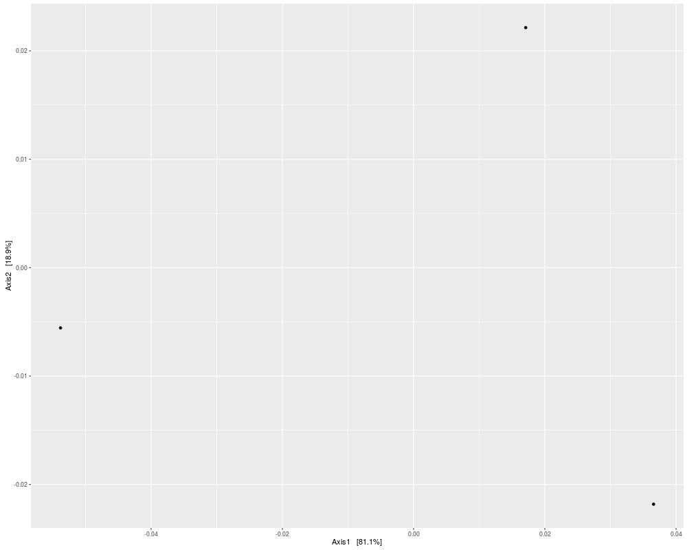
> plot_ordination(esophagus, eso.dpcoa, "samples")
No available covariate data to map on the points for this plot `type`
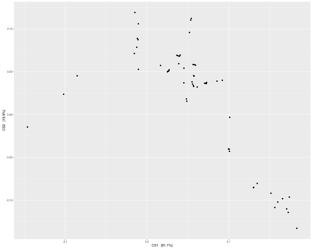
> plot_ordination(esophagus, eso.dpcoa, "species")
No available covariate data to map on the points for this plot `type`
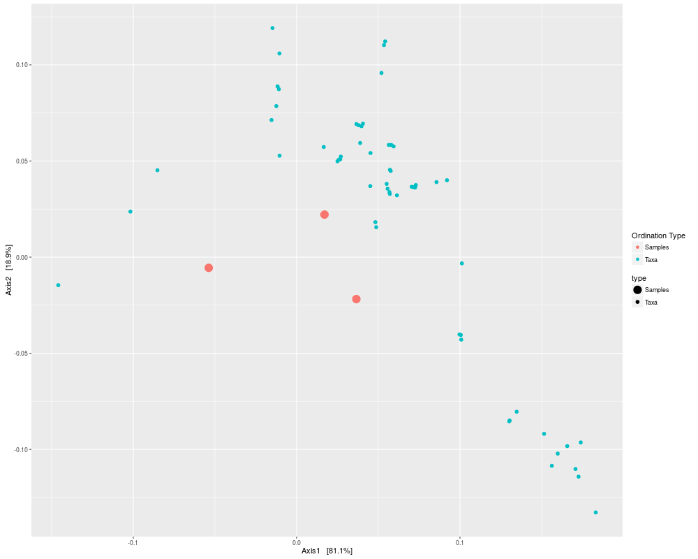
> plot_ordination(esophagus, eso.dpcoa, "biplot")
> #
> #
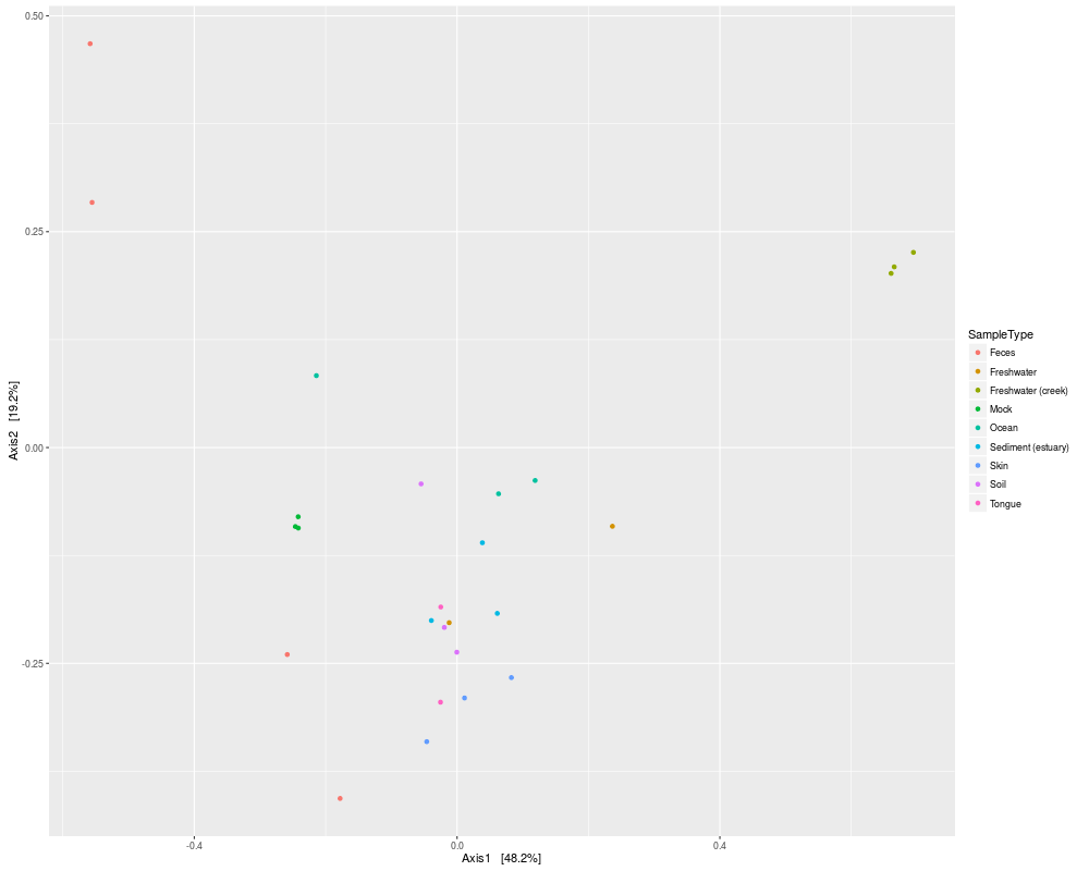
> # # # # # # GlobalPatterns
> data(GlobalPatterns)
> # subset GP to top-150 taxa (to save computation time in example)
> keepTaxa <- names(sort(taxa_sums(GlobalPatterns), TRUE)[1:150])
> GP       <- prune_taxa(keepTaxa, GlobalPatterns)
> # Perform DPCoA
> GP.dpcoa <- DPCoA(GP)
> plot_ordination(GP, GP.dpcoa, color="SampleType")
> 
> 
> 
> 
> 
> dev.off()
null device 
          1 
>