Create a ggplot summary of gap statistic results

Description

Create a ggplot summary of gap statistic results

Usage

plot_clusgap(clusgap, title = "Gap Statistic results")

Arguments

Value

A ggplot plot object. The rendered graphic should be a plot of the gap statistic score versus values for k, the number of clusters.

See Also

gapstat_ord

clusGap

ggplot

Examples

# Load and process data
data("soilrep")
soilr = rarefy_even_depth(soilrep, rngseed=888)
print(soilr)
sample_variables(soilr)
# Ordination
sord  = ordinate(soilr, "DCA")
# Gap Statistic
gs = gapstat_ord(sord, axes=1:4, verbose=FALSE)
# Evaluate results with plots, etc.
plot_scree(sord)
plot_ordination(soilr, sord,  color="Treatment")
plot_clusgap(gs)
print(gs, method="Tibs2001SEmax")
# Non-ordination example, use cluster::clusGap function directly
library("cluster")
pam1 = function(x, k){list(cluster = pam(x, k, cluster.only=TRUE))}
gs.pam.RU = clusGap(ruspini, FUN = pam1, K.max = 8, B = 60)
gs.pam.RU
plot(gs.pam.RU, main = "Gap statistic for the 'ruspini' data")
mtext("k = 4 is best .. and  k = 5  pretty close")
plot_clusgap(gs.pam.RU)

Results

R version 3.3.1 (2016-06-21) -- "Bug in Your Hair"
Copyright (C) 2016 The R Foundation for Statistical Computing
Platform: x86_64-pc-linux-gnu (64-bit)

R is free software and comes with ABSOLUTELY NO WARRANTY.
You are welcome to redistribute it under certain conditions.
Type 'license()' or 'licence()' for distribution details.

R is a collaborative project with many contributors.
Type 'contributors()' for more information and
'citation()' on how to cite R or R packages in publications.

Type 'demo()' for some demos, 'help()' for on-line help, or
'help.start()' for an HTML browser interface to help.
Type 'q()' to quit R.

> library(phyloseq)
> png(filename="/home/ddbj/snapshot/RGM3/R_BC/result/phyloseq/plot_clusgap.Rd_%03d_medium.png", width=480, height=480)
> ### Name: plot_clusgap
> ### Title: Create a ggplot summary of gap statistic results
> ### Aliases: plot_clusgap
> 
> ### ** Examples
> 
> # Load and process data
> data("soilrep")
> soilr = rarefy_even_depth(soilrep, rngseed=888)
`set.seed(888)` was used to initialize repeatable random subsampling.
Please record this for your records so others can reproduce.
Try `set.seed(888); .Random.seed` for the full vector
...
5510OTUs were removed because they are no longer 
present in any sample after random subsampling

...
> print(soilr)
phyloseq-class experiment-level object
otu_table()   OTU Table:         [ 11315 taxa and 56 samples ]
sample_data() Sample Data:       [ 56 samples by 4 sample variables ]
> sample_variables(soilr)
[1] "Treatment" "warmed"    "clipped"   "Sample"   
> # Ordination
> sord  = ordinate(soilr, "DCA")
> # Gap Statistic
> gs = gapstat_ord(sord, axes=1:4, verbose=FALSE)
> # Evaluate results with plots, etc.
> plot_scree(sord)
> plot_ordination(soilr, sord,  color="Treatment")
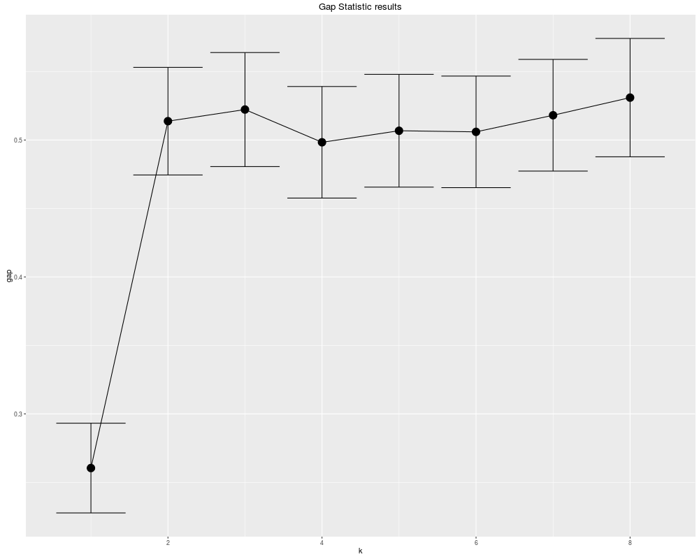
> plot_clusgap(gs)
> print(gs, method="Tibs2001SEmax")
Clustering Gap statistic ["clusGap"].
B=100 simulated reference sets, k = 1..8
 --> Number of clusters (method 'Tibs2001SEmax', SE.factor=1): 2
         logW   E.logW       gap     SE.sim
[1,] 3.352519 3.612945 0.2604261 0.03276793
[2,] 2.952424 3.466195 0.5137715 0.03929898
[3,] 2.823440 3.345692 0.5222520 0.04163931
[4,] 2.740943 3.239285 0.4983427 0.04073436
[5,] 2.639522 3.146296 0.5067739 0.04118294
[6,] 2.558331 3.064290 0.5059582 0.04074180
[7,] 2.471036 2.989125 0.5180888 0.04077731
[8,] 2.390007 2.920966 0.5309587 0.04322675
> # Non-ordination example, use cluster::clusGap function directly
> library("cluster")
> pam1 = function(x, k){list(cluster = pam(x, k, cluster.only=TRUE))}
> gs.pam.RU = clusGap(ruspini, FUN = pam1, K.max = 8, B = 60)
> gs.pam.RU
Clustering Gap statistic ["clusGap"].
B=60 simulated reference sets, k = 1..8
 --> Number of clusters (method 'firstSEmax', SE.factor=1): 4
         logW   E.logW         gap     SE.sim
[1,] 7.187997 7.139770 -0.04822666 0.04335827
[2,] 6.628498 6.784040  0.15554220 0.04497106
[3,] 6.261660 6.575423  0.31376306 0.05415527
[4,] 5.692736 6.389210  0.69647353 0.05961542
[5,] 5.580999 6.245714  0.66471515 0.05030286
[6,] 5.500583 6.119008  0.61842460 0.04107241
[7,] 5.394195 6.010613  0.61641841 0.04174399
[8,] 5.320052 5.917322  0.59726968 0.04432359
> plot(gs.pam.RU, main = "Gap statistic for the 'ruspini' data")
> mtext("k = 4 is best .. and  k = 5  pretty close")
> plot_clusgap(gs.pam.RU)
> 
> 
> 
> 
> 
> dev.off()
null device 
          1 
>