R Graphical Manual

Browse All

Last data update: 2014.03.03

R: Dependency score plotting

plot	R Documentation

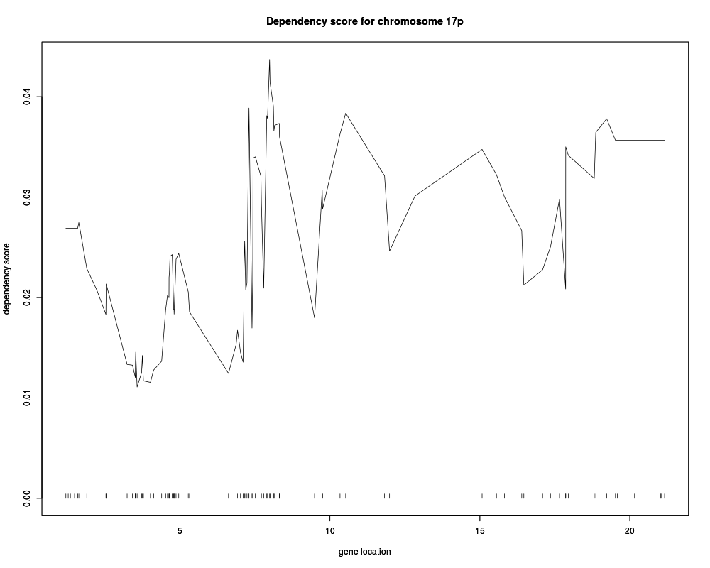
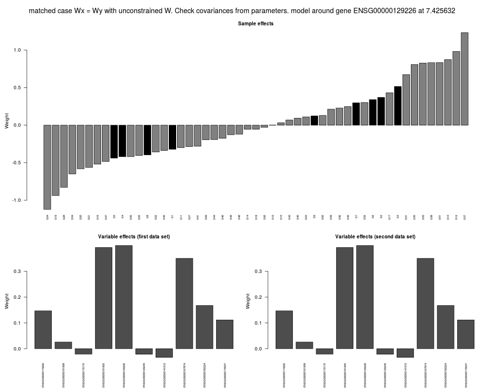
Dependency score plotting

Description

Plot the contribution of the samples and variables to the dependency model or dependency model fitting scores of chromosome or genome.

Usage

## S3 method for class 'GeneDependencyModel'
plot(x, X, Y, ann.types = NULL, ann.cols = NULL, legend.x = 0, 
        legend.y = 1, legend.xjust = 0, legend.yjust = 1, order = FALSE, 
        cex.z = 0.6, cex.WX = 0.6, cex.WY = 0.6, ...)


## S3 method for class 'ChromosomeModels'
plot(x, hilightGenes = NULL, showDensity = FALSE, showTop = 0,
	topName = FALSE, type = 'l', xlab = 'gene location', ylab = 'dependency score',
	main = NULL,
	pch = 20, cex = 0.75, tpch = 3, tcex = 1, xlim = NA, ylim = NA,...)

## S3 method for class 'GenomeModels'
plot(x, hilightGenes = NULL, showDensity = FALSE, showTop = 0, 
	topName = FALSE, onePlot = FALSE, type = 'l', ylab = "Dependency Scores", 
	xlab = "Gene location (chromosome)", main = "Dependency Scores in All Chromosomes",
	pch = 20, cex = 0.75, tpch = 20, tcex = 0.7, mfrow = c(5,5), mar = c(3,2.5,1.3,0.5), 
	ps = 5, mgp = c(1.5,0.5,0),ylim=NA,...)

Arguments

`x`	`GeneDependencyModel-class`, `ChromosomeModels-class`, `GenomeModels-class`; models to be plotted.
`X, Y`	data sets used in dependency modeling.
`ann.types`	a factor for annotation types for samples. Each value corresponds one sample in datasets. Colors are used to indicate different types.
`ann.cols`	colors used to indicate different annotation types. Gray scale is used if 'NULL' given.
`legend.x, legend.y`	the x and y co-ordinates to be used to position the legend for annotation types.
`legend.xjust, legend.yjust`	how the legend is to be justified relative to the legend x and y location. A value of 0 means left or top justified, 0.5 means centered and 1 means right or bottom justified.
`order`	logical; if 'TRUE', values for sample contributions are ordered according to their values.
`cex.z, cex.WX, cex.WY`	Text size for variable names.
`hilightGenes`	vector of strings; Name of genes to be hilighted with dots.
`showDensity`	logical; if 'TRUE' small vertical lines are drwan in the bottom of the plot under each gene.
`showTop`	numeric; Number of models with highest dependencies to be hilighted. A horizontal dashed line is drawn to show threshold value. With `0` no line is drawn.
`topName`	logical; If `TRUE`, gene names are printed to hilighted models with highest dependecies. Otherwise hilighted models are numbered according to their rank in dependency score.
`type, xlab, ylab, main`	plot type and labels. See `plot` for details. A text for chromosome (and arm if only models from one arm is plotted) is used in `main` if `NULL` is given. In `plot.GenomeModels`, `ylab` and `xlab` affect only if `onePlot` is `TRUE`.
`onePlot`	If `TRUE`, all dependency scores are plotted in one plot window. Otherwise one plot window is used for each chromosome.
`pch, cex`	symbol type and size for hilightGenes. See `points` for details.
`tpch, tcex`	symbol type and size for genes with highest scores. See `points` for details.
`ylim, xlim`	axis limits. Default values are calculated from data. Lower limit for y is 0 and upper limit is either 1 or maximum score value. X limits are gene location range. See `plot` for details.
`mfrow, mar, ps, mgp`	chromosome plots' layout, marginals, text size and margin line. See `par` for details.
`...`	optional plotting parameters

Details

Function plots scores of each dependency model of a gene for the whole chromosome or genome according to used method. plot(x, cancerGenes = NULL, showDensity = FALSE, ...) is also usable and chosen according to class of models.

Author(s)

Olli-Pekka Huovilainen ohuovila@gmail.com

References

Dependency Detection with Similarity Constraints Lahti et al., MLSP'09. See http://www.cis.hut.fi/lmlahti/publications/mlsp09_preprint.pdf

Examples


data(chromosome17)

## pSimCCA model on chromosome 17p
models17ppSimCCA <- screen.cgh.mrna(geneExp, geneCopyNum, 10, 17, 'p')
plot(models17ppSimCCA,
     hilightGenes=c("ENSG00000108342", "ENSG00000108298"), showDensity = TRUE)

## Dependency model around 50th gene
model <- models17ppSimCCA[[50]]

## example annnotation types
ann.types <- factor(c(rep("Samples 1 - 10", 10), rep("Samples 11 - 51", 41)))
plot(model, geneExp, geneCopyNum, ann.types, legend.x = 40, legend.y = -4,
     order = TRUE)

Results


R version 3.3.1 (2016-06-21) -- "Bug in Your Hair"
Copyright (C) 2016 The R Foundation for Statistical Computing
Platform: x86_64-pc-linux-gnu (64-bit)

R is free software and comes with ABSOLUTELY NO WARRANTY.
You are welcome to redistribute it under certain conditions.
Type 'license()' or 'licence()' for distribution details.

R is a collaborative project with many contributors.
Type 'contributors()' for more information and
'citation()' on how to cite R or R packages in publications.

Type 'demo()' for some demos, 'help()' for on-line help, or
'help.start()' for an HTML browser interface to help.
Type 'q()' to quit R.

> library(pint)
Loading required package: mvtnorm
Loading required package: Matrix
Loading required package: dmt
Loading required package: MASS

dmt Copyright (C) 2008-2013 Leo Lahti and Olli-Pekka Huovilainen.
This program comes with ABSOLUTELY NO
WARRANTY.
This is free software, and you are welcome to redistribute it
under the FreeBSD license.



pint Copyright (C) 2008-2013 Olli-Pekka Huovilainen and Leo Lahti.

This program comes with ABSOLUTELY NO WARRANTY.
This is free software, and you are welcome to redistribute it
under the FreeBSD license.

> png(filename="/home/ddbj/snapshot/RGM3/R_BC/result/pint/plot.Rd_%03d_medium.png", width=480, height=480)
> ### Name: plot
> ### Title: Dependency score plotting
> ### Aliases: plot.GeneDependencyModel plot.ChromosomeModels
> ###   plot.GenomeModels 'dependency score plotting'
> ### Keywords: hplot
> 
> ### ** Examples
> 
> 
> data(chromosome17)
> 
> ## pSimCCA model on chromosome 17p
> models17ppSimCCA <- screen.cgh.mrna(geneExp, geneCopyNum, 10, 17, 'p')
Imputing missing values..
Imputing missing values..
Matching probes between the data sets..
Calculating dependency models for 17p with method pSimCCA, window size:10
17p; window 1/92
17p; window 2/92
17p; window 3/92
17p; window 4/92
17p; window 5/92
17p; window 6/92
17p; window 7/92
17p; window 8/92
17p; window 9/92
17p; window 10/92
17p; window 11/92
17p; window 12/92
17p; window 13/92
17p; window 14/92
17p; window 15/92
17p; window 16/92
17p; window 17/92
17p; window 18/92
17p; window 19/92
17p; window 20/92
17p; window 21/92
17p; window 22/92
17p; window 23/92
17p; window 24/92
17p; window 25/92
17p; window 26/92
17p; window 27/92
17p; window 28/92
17p; window 29/92
17p; window 30/92
17p; window 31/92
17p; window 32/92
17p; window 33/92
17p; window 34/92
17p; window 35/92
17p; window 36/92
17p; window 37/92
17p; window 38/92
17p; window 39/92
17p; window 40/92
17p; window 41/92
17p; window 42/92
17p; window 43/92
17p; window 44/92
17p; window 45/92
17p; window 46/92
17p; window 47/92
17p; window 48/92
17p; window 49/92
17p; window 50/92
17p; window 51/92
17p; window 52/92
17p; window 53/92
17p; window 54/92
17p; window 55/92
17p; window 56/92
17p; window 57/92
17p; window 58/92
17p; window 59/92
17p; window 60/92
17p; window 61/92
17p; window 62/92
17p; window 63/92
17p; window 64/92
17p; window 65/92
17p; window 66/92
17p; window 67/92
17p; window 68/92
17p; window 69/92
17p; window 70/92
17p; window 71/92
17p; window 72/92
17p; window 73/92
17p; window 74/92
17p; window 75/92
17p; window 76/92
17p; window 77/92
17p; window 78/92
17p; window 79/92
17p; window 80/92
17p; window 81/92
17p; window 82/92
17p; window 83/92
17p; window 84/92
17p; window 85/92
17p; window 86/92
17p; window 87/92
17p; window 88/92
17p; window 89/92
17p; window 90/92
17p; window 91/92
17p; window 92/92
> plot(models17ppSimCCA,
+      hilightGenes=c("ENSG00000108342", "ENSG00000108298"), showDensity = TRUE)
> 
> ## Dependency model around 50th gene
> model <- models17ppSimCCA[[50]]
> 
> ## example annnotation types
> ann.types <- factor(c(rep("Samples 1 - 10", 10), rep("Samples 11 - 51", 41)))
> plot(model, geneExp, geneCopyNum, ann.types, legend.x = 40, legend.y = -4,
+      order = TRUE)
> 
> 
> 
> 
> 
> 
> 
> dev.off()
null device 
          1 
>