R Graphical Manual

Browse All

Last data update: 2014.03.03

R: Computed ABC analysis: calculates a division of the data in 3...

ABCanalysis

R Documentation

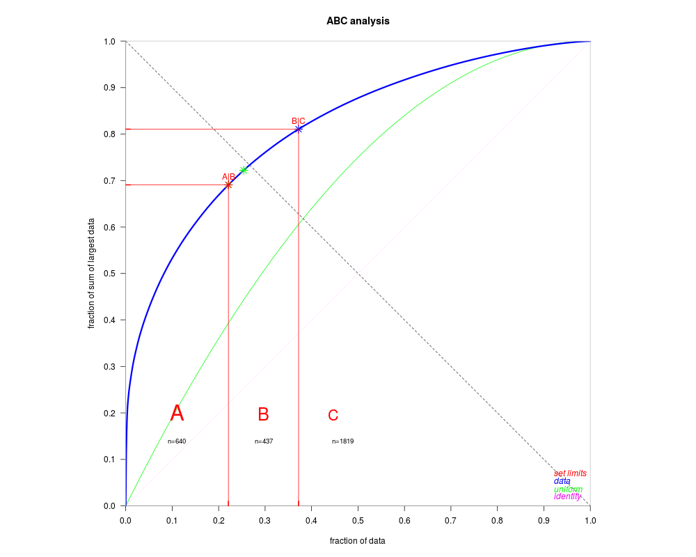
Computed ABC analysis: calculates a division of the data in 3 classes A, B and C

Description

divide the Data in 3 classes A, B and C such that

A=Data[Aind] : with low effort much yield

B=Data[Bind] : yield and effort are about equal

C=Data[Cind] : with much effort low yield

Usage

ABCanalysis(Data,PlotIt,ABCcurvedata)

Arguments

`Data`	vector(1:n) describes an array of data: n cases in rows of one variable, if matrix or dataframe then first column will be used.
`PlotIt`	if variable is used, a plot is made, set with arbitrary value
`ABCcurvedata`	only for internal usage, list from ABCcurve

Details

Pareto point: Minimum distance to (0,1) = minimal unrealized potential

BreakEven Point: B_x is the x value of the point, where the slope of ABCcurve equals one.

For further description to p in variable AlimitIndInInterpolation see ABCcurve

Value

Output is of type list which parts are described in the following

`Aind`	vector [1:j], A==Data(Aind) : with little effort much Yield
`Bind`	vector [1:l], B==Data(Bind) : effort and Yield are balanced
`Cind`	(vector [1:m], C==Data(Cind) : much effort for little Yield
`ABexchanged`	Boolean, TRUE if Point A is the Break Even and point B is the Pareto Point, FALSE otherwise
`A`	c(Ax,Ay), Pareto point or BreakEven Point indicated by ABexchanged
`B`	c(Bx,By), Pareto point or BreakEven Point indicated by ABexchanged
`C`	Submarginal point: minimum distance to `[B_x,1]`
`smallestAData`	Boundary AB, defined by point A or B with ABexchanged
`smallestBData`	Boundary BC, defined by point C
`AlimitIndInInterpolation`	index of AB Boundary in [`p`, ABC], the interpolation of the ABC plot
`BlimitIndInInterpolation`	index of BC Boundary in [`p`, ABC], the interpolation of the ABC plot

Author(s)

Michael Thrun

http://www.uni-marburg.de/fb12/datenbionik

References

Ultsch. A ., Lotsch J.: Computed ABC Analysis for rational Selection of most informative Variables in multivariate Data, PLoS One, Jun 10, 10(6), e0129767, 2015.

Examples

  data("SwissInhabitants")
	abc=ABCanalysis(SwissInhabitants,PlotIt=TRUE)
	A=abc$Aind
	B=abc$Bind
	C=abc$Cind
	Agroup=SwissInhabitants[A]
	Bgroup=SwissInhabitants[B]
	Cgroup=SwissInhabitants[C]

Results


R version 3.3.1 (2016-06-21) -- "Bug in Your Hair"
Copyright (C) 2016 The R Foundation for Statistical Computing
Platform: x86_64-pc-linux-gnu (64-bit)

R is free software and comes with ABSOLUTELY NO WARRANTY.
You are welcome to redistribute it under certain conditions.
Type 'license()' or 'licence()' for distribution details.

R is a collaborative project with many contributors.
Type 'contributors()' for more information and
'citation()' on how to cite R or R packages in publications.

Type 'demo()' for some demos, 'help()' for on-line help, or
'help.start()' for an HTML browser interface to help.
Type 'q()' to quit R.

> library(ABCanalysis)
> png(filename="/home/ddbj/snapshot/RGM3/R_CC/result/ABCanalysis/ABCanalysis.Rd_%03d_medium.png", width=480, height=480)
> ### Name: ABCanalysis
> ### Title: Computed ABC analysis: calculates a division of the data in 3
> ###   classes A, B and C
> ### Aliases: ABCanalysis
> ### Keywords: ABC ABCanalysis ABC analysis Lorenz curve Lorenz
> 
> ### ** Examples
> 
>   data("SwissInhabitants")
> 	abc=ABCanalysis(SwissInhabitants,PlotIt=TRUE)
> 	A=abc$Aind
> 	B=abc$Bind
> 	C=abc$Cind
> 	Agroup=SwissInhabitants[A]
> 	Bgroup=SwissInhabitants[B]
> 	Cgroup=SwissInhabitants[C]
> 
> 
> 
> 
> 
> 
> dev.off()
null device 
          1 
>