R Graphical Manual

Browse All

Last data update: 2014.03.03

R: Abrupt Change-Point or Aberration Detection in a Series of...

ACA-package

R Documentation

Abrupt Change-Point or Aberration Detection in a Series of Points

Description

Offers an interactive function for the detection of breakpoints in series.

Details

Package:	ACA
Type:	Package
Version:	1.0
Date:	2016-03-08
License:	GPL
LazyLoad:	yes

Author(s)

Daniel Amorese <amorese@ipgp.fr>,

Maintainer: Daniel Amorese <amorese@ipgp.fr>

References

D. Amorese, "Applying a change-point detection method on frequency-magnitude distributions", Bull. seism. Soc. Am. (2007) 97, doi:10.1785/0120060181

Lanzante, J. R., "Resistant, robust and non-parametric techniques for the analysis of climate data: Theory and examples, including applications to historical radiosonde station data", International Journal of Climatology (1996) 16(11), 1197-1226

Examples

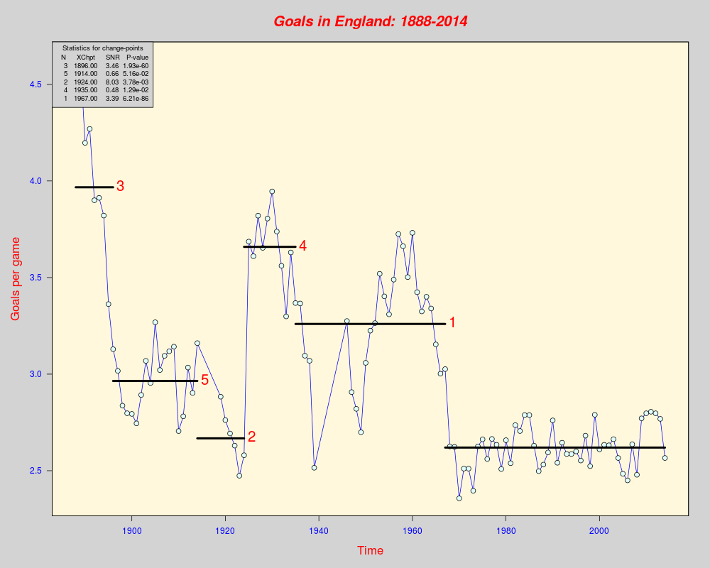
    SDScan(namefi=system.file("extdata","soccer.data.txt",package="ACA"),
    xleg="Time", yleg="Goals per game", titl="Goals in England: 1888-2014", onecol="n", daty="n")

Results


R version 3.3.1 (2016-06-21) -- "Bug in Your Hair"
Copyright (C) 2016 The R Foundation for Statistical Computing
Platform: x86_64-pc-linux-gnu (64-bit)

R is free software and comes with ABSOLUTELY NO WARRANTY.
You are welcome to redistribute it under certain conditions.
Type 'license()' or 'licence()' for distribution details.

R is a collaborative project with many contributors.
Type 'contributors()' for more information and
'citation()' on how to cite R or R packages in publications.

Type 'demo()' for some demos, 'help()' for on-line help, or
'help.start()' for an HTML browser interface to help.
Type 'q()' to quit R.

> library(ACA)
> png(filename="/home/ddbj/snapshot/RGM3/R_CC/result/ACA/ACA-package.Rd_%03d_medium.png", width=480, height=480)
> ### Name: ACA-package
> ### Title: Abrupt Change-Point or Aberration Detection in a Series of
> ###   Points
> ### Aliases: ACA-package ACA
> ### Keywords: package
> 
> ### ** Examples
> 
>     SDScan(namefi=system.file("extdata","soccer.data.txt",package="ACA"),
+     xleg="Time", yleg="Goals per game", titl="Goals in England: 1888-2014", onecol="n", daty="n")

*************************************************************************************

Serial Data Scanner V1.5 

R function for change-point detection through the Lanzante's method (Lanzante,1996)

J. R. Lanzante, (1996). Resistant, robust and non-parametric techniques for the
analysis of climate data : theory and examples, including applications to
historical radiosonde station data, International Journal of Climatology,
vol. 16, 1197-1226.

Other reference : D. Amorese, (2007). Applying a change-point detection method
on frequency-magnitude distributions, Bulletin of the Seismological Society of
America, 97(5):1742-1749

*************************************************************************************

Change-point detection is being performed

ITERATION # 1 


n1= 70 W= 5581.5 

 niter= 1n= 117 n2= 47 Critical W= 4130 
sw= 179.8657 sw_t= 179.8633 W= 5581.5 Wx= 1392 
p-value = 7.19073e-16 ntau_i = 70 
	Test Passed

nxbar= 44.22857 nybar= 4.106383 sdnx= 4780.343 sdny= 496.4681 zstat= 19.64641 p= 6.205218e-86 
	Robust Rank Order Test Passed

MEDPAIRWISE : 97 points ->  4656 2-points slopes

	slope= -0.006538906 intercept= 15.69604 

snr -> xl= 3.23534 n= 50 nl= 20 xr= 2.619704 n= 47 nr= 117 x= 2.937042 sd= 0.09564707 sn= 0.07061163 snr= 0.07061163 

MEDPAIRWISE : 97 points ->  4656 2-points slopes

	slope= -0.006538906 intercept= 15.69604 

b= -0.006538906 A= 15.69604 

snr -> xl= 3.23534 n= 50 nl= 20 xr= 2.619704 n= 47 nr= 117 x= 2.937042 sd= 0.09564707 sn= 0.1387135 snr= 0.1387135 

Disc. Noise Var.= 0.07061163 Trend Noise Var= 0.1387135 

 70 <->  1  117
Gap between change-points
CHANGE-POINT DETECTED

ADJUSTMENT # 1
ITERATION # 1 


n1= 33 W= 1389 

 niter= 1n= 117 n2= 84 Critical W= 1947 
sw= 165.1 sw_t= 165.0981 W= 1389 Wx= 1389 
p-value = 0.000733397 ntau_i = 33 
	Test Passed

nxbar= 25.09091 nybar= 23.14286 sdnx= 34766.73 sdny= 1776.286 zstat= -2.896067 p= 0.003778714 
	Robust Rank Order Test Passed

MEDPAIRWISE : 70 points ->  2415 2-points slopes

	slope= -0.0003148022 intercept= 3.853703 

snr -> xl= 3.022943 n= 33 nl= 1 xr= 3.372143 n= 37 nr= 70 x= 3.20752 sd= 0.03082587 sn= 0.1396428 snr= 0.1396428 

MEDPAIRWISE : 70 points ->  2415 2-points slopes

	slope= -0.0003148022 intercept= 3.853703 

b= -0.0003148022 A= 3.853703 

snr -> xl= 3.022943 n= 33 nl= 1 xr= 3.372143 n= 37 nr= 70 x= 3.20752 sd= 0.03082587 sn= 0.2137295 snr= 0.2137295 

Disc. Noise Var.= 0.1396428 Trend Noise Var= 0.2137295 

 33 <->  1  117  70
Gap between change-points
CHANGE-POINT DETECTED

ADJUSTMENT # 2
ITERATION # 1 


n1= 9 W= 983 

 niter= 1n= 117 n2= 108 Critical W= 531 
sw= 97.76502 sw_t= 97.76209 W= 983 Wx= 983 
p-value = 3.867952e-06 ntau_i = 9 
	Test Passed

nxbar= 104.2222 nybar= 0.3148148 sdnx= 691.5556 sdny= 35.2963 zstat= 16.3994 p= 1.931221e-60 
	Robust Rank Order Test Passed

MEDPAIRWISE : 33 points ->  528 2-points slopes

	slope= -0.037753 intercept= 75.15114 

snr -> xl= 3.967118 n= 9 nl= 1 xr= 2.890656 n= 24 nr= 33 x= 3.184237 sd= 0.2370212 sn= 0.07667512 snr= 0.07667512 

MEDPAIRWISE : 33 points ->  528 2-points slopes

	slope= -0.037753 intercept= 75.15114 

b= -0.037753 A= 75.15114 

snr -> xl= 3.967118 n= 9 nl= 1 xr= 2.890656 n= 24 nr= 33 x= 3.184237 sd= 0.2370212 sn= 0.1460344 snr= 0.1460344 

Disc. Noise Var.= 0.07667512 Trend Noise Var= 0.1460344 

 9 <->  1  117  70  33
Gap between change-points
CHANGE-POINT DETECTED

ADJUSTMENT # 3
ITERATION # 1 


n1= 44 W= 3057 

 niter= 1n= 117 n2= 73 Critical W= 2596 
sw= 177.7208 sw_t= 177.7154 W= 3057 Wx= 3057 
p-value = 0.009563597 ntau_i = 44 
	Test Passed

nxbar= 46.93182 nybar= 15.65753 sdnx= 28426.8 sdny= 5222.438 zstat= 2.486121 p= 0.0129144 
	Robust Rank Order Test Passed

MEDPAIRWISE : 37 points ->  666 2-points slopes

	slope= -0.00890429 intercept= 20.76369 

snr -> xl= 3.658781 n= 11 nl= 33 xr= 3.25975 n= 26 nr= 70 x= 3.378381 sd= 0.03418811 sn= 0.0711182 snr= 0.0711182 

MEDPAIRWISE : 37 points ->  666 2-points slopes

	slope= -0.00890429 intercept= 20.76369 

b= -0.00890429 A= 20.76369 

snr -> xl= 3.658781 n= 11 nl= 33 xr= 3.25975 n= 26 nr= 70 x= 3.378381 sd= 0.03418811 sn= 0.08692649 snr= 0.08692649 

Disc. Noise Var.= 0.0711182 Trend Noise Var= 0.08692649 

 44 <->  1  117  70  33  9
Gap between change-points
CHANGE-POINT DETECTED

ADJUSTMENT # 4
ITERATION # 1 


n1= 27 W= 1912.5 

 niter= 1n= 117 n2= 90 Critical W= 1593 
sw= 154.5801 sw_t= 154.5757 W= 1912.5 Wx= 1912.5 
p-value = 0.0390449 ntau_i = 27 
	Test Passed

nxbar= 56.77778 nybar= 9.933333 sdnx= 23028.67 sdny= 3343.6 zstat= 1.946714 p= 0.051569 

MEDPAIRWISE : 24 points ->  276 2-points slopes

	slope= -0.008929573 intercept= 19.93138 

snr -> xl= 2.96462 n= 18 nl= 9 xr= 2.667487 n= 6 nr= 33 x= 2.890337 sd= 0.01727371 sn= 0.02613829 snr= 0.02613829 

MEDPAIRWISE : 24 points ->  276 2-points slopes

	slope= -0.008929573 intercept= 19.93138 

b= -0.008929573 A= 19.93138 

snr -> xl= 2.96462 n= 18 nl= 9 xr= 2.667487 n= 6 nr= 33 x= 2.890337 sd= 0.01727371 sn= 0.03445906 snr= 0.03445906 

Disc. Noise Var.= 0.02613829 Trend Noise Var= 0.03445906 

 27 <->  1  117  70  33  9  44
Gap between change-points
CHANGE-POINT DETECTED

ADJUSTMENT # 5
ITERATION # 1 


n1= 55 W= 2955 

 niter= 1n= 117 n2= 62 Critical W= 3245 
sw= 183.1165 sw_t= 183.1114 W= 2955 Wx= 2955 
p-value = 0.1138769 ntau_i = 55 

ITERATION # 2 


n1= 54 W= 2904 

 niter= 2n= 117 n2= 63 Critical W= 3186 
sw= 182.9016 sw_t= 182.8965 W= 2904 Wx= 2904 
p-value = 0.1237745 ntau_i = 54 

ITERATION # 3 


n1= 53 W= 2863 

 niter= 3n= 117 n2= 64 Critical W= 3127 
sw= 182.6326 sw_t= 182.6275 W= 2863 Wx= 2863 
p-value = 0.149069 ntau_i = 53 

ITERATION # 4 


n1= 56 W= 3063 

 niter= 4n= 117 n2= 61 Critical W= 3304 
sw= 183.2776 sw_t= 183.2724 W= 3063 Wx= 3063 
p-value = 0.1894344 ntau_i = 56 

ITERATION # 5 


n1= 52 W= 2849 

 niter= 5n= 117 n2= 65 Critical W= 3068 
sw= 182.3093 sw_t= 182.3041 W= 2849 Wx= 2849 
p-value = 0.2307043 ntau_i = 52 

NUMBER OF ITERATIONS : 5
MEDPAIRWISE : 73 points ->  2628 2-points slopes

	slope= -0.007690945 intercept= 17.99242 

snr -> xl= 3.25975 n= 26 nl= 44 xr= 2.619704 n= 47 nr= 117 x= 2.847666 sd= 0.09524398 sn= 0.02805443 snr= 0.02805443 

MEDPAIRWISE : 73 points ->  2628 2-points slopes

	slope= -0.007690945 intercept= 17.99242 

b= -0.007690945 A= 17.99242 

snr -> xl= 3.25975 n= 26 nl= 44 xr= 2.619704 n= 47 nr= 117 x= 2.847666 sd= 0.09524398 sn= 0.0828115 snr= 0.0828115 

MEDPAIRWISE : 73 points ->  2628 2-points slopes

	slope= -0.007690945 intercept= 17.99242 

snr -> xl= 3.25975 n= 26 nl= 44 xr= 2.619704 n= 47 nr= 117 x= 2.847666 sd= 0.09524398 sn= 0.02805443 snr= 3.394971 

MEDPAIRWISE : 17 points ->  136 2-points slopes

	slope= 0.0520313 intercept= -96.96495 

snr -> xl= 2.667487 n= 6 nl= 27 xr= 3.658781 n= 11 nr= 44 x= 3.308913 sd= 0.2384404 sn= 0.02969497 snr= 0.02969497 

MEDPAIRWISE : 17 points ->  136 2-points slopes

	slope= 0.0520313 intercept= -96.96495 

b= 0.0520313 A= -96.96495 

snr -> xl= 2.667487 n= 6 nl= 27 xr= 3.658781 n= 11 nr= 44 x= 3.308913 sd= 0.2384404 sn= 0.1588658 snr= 0.1588658 

MEDPAIRWISE : 17 points ->  136 2-points slopes

	slope= 0.0520313 intercept= -96.96495 

snr -> xl= 2.667487 n= 6 nl= 27 xr= 3.658781 n= 11 nr= 44 x= 3.308913 sd= 0.2384404 sn= 0.02969497 snr= 8.029655 

MEDPAIRWISE : 27 points ->  351 2-points slopes

	slope= -0.04884868 intercept= 96.24918 

snr -> xl= 3.967118 n= 9 nl= 1 xr= 2.96462 n= 18 nr= 27 x= 3.298786 sd= 0.2319237 sn= 0.06710097 snr= 0.06710097 

MEDPAIRWISE : 27 points ->  351 2-points slopes

	slope= -0.04884868 intercept= 96.24918 

b= -0.04884868 A= 96.24918 

snr -> xl= 3.967118 n= 9 nl= 1 xr= 2.96462 n= 18 nr= 27 x= 3.298786 sd= 0.2319237 sn= 0.1671598 snr= 0.1671598 

MEDPAIRWISE : 27 points ->  351 2-points slopes

	slope= -0.04884868 intercept= 96.24918 

snr -> xl= 3.967118 n= 9 nl= 1 xr= 2.96462 n= 18 nr= 27 x= 3.298786 sd= 0.2319237 sn= 0.06710097 snr= 3.456338 

MEDPAIRWISE : 37 points ->  666 2-points slopes

	slope= -0.00890429 intercept= 20.76369 

snr -> xl= 3.658781 n= 11 nl= 33 xr= 3.25975 n= 26 nr= 70 x= 3.378381 sd= 0.03418811 sn= 0.0711182 snr= 0.0711182 

MEDPAIRWISE : 37 points ->  666 2-points slopes

	slope= -0.00890429 intercept= 20.76369 

b= -0.00890429 A= 20.76369 

snr -> xl= 3.658781 n= 11 nl= 33 xr= 3.25975 n= 26 nr= 70 x= 3.378381 sd= 0.03418811 sn= 0.08692649 snr= 0.08692649 

MEDPAIRWISE : 37 points ->  666 2-points slopes

	slope= -0.00890429 intercept= 20.76369 

snr -> xl= 3.658781 n= 11 nl= 33 xr= 3.25975 n= 26 nr= 70 x= 3.378381 sd= 0.03418811 sn= 0.0711182 snr= 0.4807224 

MEDPAIRWISE : 24 points ->  276 2-points slopes

	slope= -0.008929573 intercept= 19.93138 

snr -> xl= 2.96462 n= 18 nl= 9 xr= 2.667487 n= 6 nr= 33 x= 2.890337 sd= 0.01727371 sn= 0.02613829 snr= 0.02613829 

MEDPAIRWISE : 24 points ->  276 2-points slopes

	slope= -0.008929573 intercept= 19.93138 

b= -0.008929573 A= 19.93138 

snr -> xl= 2.96462 n= 18 nl= 9 xr= 2.667487 n= 6 nr= 33 x= 2.890337 sd= 0.01727371 sn= 0.03445906 snr= 0.03445906 

MEDPAIRWISE : 24 points ->  276 2-points slopes

	slope= -0.008929573 intercept= 19.93138 

snr -> xl= 2.96462 n= 18 nl= 9 xr= 2.667487 n= 6 nr= 33 x= 2.890337 sd= 0.01727371 sn= 0.02613829 snr= 0.6608583 

Numerical results in SDS.res


PLEASE, locate with the mouse the topright corner of the legend in the plot window

topleft
Graphics in SDS.png


Graphics in SDS.pdf

> 
> 
> 
> 
> 
> dev.off()
null device 
          1 
>