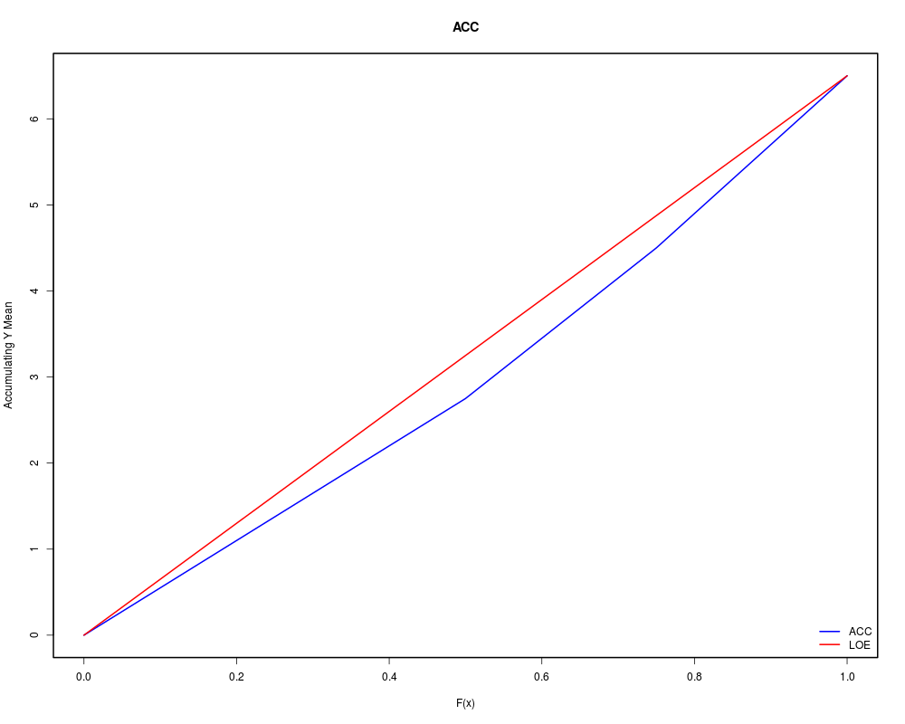
Plots the ACC vs LOI graph and the LMA graph

Description

This function receives a matrix containing the X,Y,Weight,FX,FY,LOI,LMA columns after the calcWeights and the reduceSameXs function has been used on it and plots the appropriate ACC vs LOI graph and the LMA graph, each in a seperate window

Usage

plotGraphs(mat)

Arguments

Value

none

Author(s)

Tal Carmi, Liat Gaziel

Examples

d <- c(1,1,3,4)
e <- c(5,6,7,8)
f <- c(1,1,1,1)
mydata <- data.frame(d,e,f)
names(mydata) <- c("X","Y","Weight")
mydata<-calcWeights(mydata)
mydata<-averageSameXs(mydata)
mydata<-calcFX(mydata)
mydata<-calcFY(mydata)
mydata<-calcLOI(mydata)
mydata<-calcLMA(mydata)
plotGraphs(mydata)

## The function is currently defined as
function (mat) 
{
    mat[size(mat) + 1, 4] = 0
    mat[size(mat) + 1, 5] = 0
    mat[size(mat) + 1, 6] = 0
    mat[size(mat) + 1, 7] = 0
    mat <- mat[order(mat[4]), ]
    trans <- t(mat)
    originalPar <- par(no.readonly = TRUE)
    par(lwd = 2)
    par(col = "black")
    plot(trans[4, ], trans[5, ], type = "n", main = "ACC", xlab = "F(x)", 
        ylab = "Accumulating Y Mean")
    par(col = "blue")
    lines(trans[4, ], trans[5, ], type = "l")
    par(col = "red")
    lines(trans[4, ], trans[6, ], type = "l")
    legend("bottomright", c("ACC", "LOE"), col = c("blue", "red"), 
        lwd = 2, bty = "n", text.col = "black")
    par(originalPar)
    windows()
    par(lwd = 2)
    par(col = "black")
    par(xaxs = "i")
    plot(trans[4, ], trans[7, ], type = "n", main = "LMA", xlab = "F(x)", 
        ylab = "LOE minus ACC")
    par(col = "black", lwd = 1)
    lines(c(0, 1), c(0, 0), type = "l")
    par(col = "blue", lwd = 2)
    lines(trans[4, ], trans[7, ], type = "l")
    par(originalPar)
  }

Results

R version 3.3.1 (2016-06-21) -- "Bug in Your Hair"
Copyright (C) 2016 The R Foundation for Statistical Computing
Platform: x86_64-pc-linux-gnu (64-bit)

R is free software and comes with ABSOLUTELY NO WARRANTY.
You are welcome to redistribute it under certain conditions.
Type 'license()' or 'licence()' for distribution details.

R is a collaborative project with many contributors.
Type 'contributors()' for more information and
'citation()' on how to cite R or R packages in publications.

Type 'demo()' for some demos, 'help()' for on-line help, or
'help.start()' for an HTML browser interface to help.
Type 'q()' to quit R.

> library(ACCLMA)
> png(filename="/home/ddbj/snapshot/RGM3/R_CC/result/ACCLMA/plotGraphs.Rd_%03d_medium.png", width=480, height=480)
> ### Name: plotGraphs
> ### Title: Plots the ACC vs LOI graph and the LMA graph
> ### Aliases: plotGraphs
> ### Keywords: ~kwd1 ~kwd2
> 
> ### ** Examples
> 
> d <- c(1,1,3,4)
> e <- c(5,6,7,8)
> f <- c(1,1,1,1)
> mydata <- data.frame(d,e,f)
> names(mydata) <- c("X","Y","Weight")
> mydata<-calcWeights(mydata)
> mydata<-averageSameXs(mydata)
> mydata<-calcFX(mydata)
> mydata<-calcFY(mydata)
> mydata<-calcLOI(mydata)
> mydata<-calcLMA(mydata)
> plotGraphs(mydata)
dev.new(): using pdf(file="Rplots2.pdf")
> 
> ## The function is currently defined as
> function (mat) 
+ {
+     mat[size(mat) + 1, 4] = 0
+     mat[size(mat) + 1, 5] = 0
+     mat[size(mat) + 1, 6] = 0
+     mat[size(mat) + 1, 7] = 0
+     mat <- mat[order(mat[4]), ]
+     trans <- t(mat)
+     originalPar <- par(no.readonly = TRUE)
+     par(lwd = 2)
+     par(col = "black")
+     plot(trans[4, ], trans[5, ], type = "n", main = "ACC", xlab = "F(x)", 
+         ylab = "Accumulating Y Mean")
+     par(col = "blue")
+     lines(trans[4, ], trans[5, ], type = "l")
+     par(col = "red")
+     lines(trans[4, ], trans[6, ], type = "l")
+     legend("bottomright", c("ACC", "LOE"), col = c("blue", "red"), 
+         lwd = 2, bty = "n", text.col = "black")
+     par(originalPar)
+     windows()
+     par(lwd = 2)
+     par(col = "black")
+     par(xaxs = "i")
+     plot(trans[4, ], trans[7, ], type = "n", main = "LMA", xlab = "F(x)", 
+         ylab = "LOE minus ACC")
+     par(col = "black", lwd = 1)
+     lines(c(0, 1), c(0, 0), type = "l")
+     par(col = "blue", lwd = 2)
+     lines(trans[4, ], trans[7, ], type = "l")
+     par(originalPar)
+   }
function (mat) 
{
    mat[size(mat) + 1, 4] = 0
    mat[size(mat) + 1, 5] = 0
    mat[size(mat) + 1, 6] = 0
    mat[size(mat) + 1, 7] = 0
    mat <- mat[order(mat[4]), ]
    trans <- t(mat)
    originalPar <- par(no.readonly = TRUE)
    par(lwd = 2)
    par(col = "black")
    plot(trans[4, ], trans[5, ], type = "n", main = "ACC", xlab = "F(x)", 
        ylab = "Accumulating Y Mean")
    par(col = "blue")
    lines(trans[4, ], trans[5, ], type = "l")
    par(col = "red")
    lines(trans[4, ], trans[6, ], type = "l")
    legend("bottomright", c("ACC", "LOE"), col = c("blue", "red"), 
        lwd = 2, bty = "n", text.col = "black")
    par(originalPar)
    windows()
    par(lwd = 2)
    par(col = "black")
    par(xaxs = "i")
    plot(trans[4, ], trans[7, ], type = "n", main = "LMA", xlab = "F(x)", 
        ylab = "LOE minus ACC")
    par(col = "black", lwd = 1)
    lines(c(0, 1), c(0, 0), type = "l")
    par(col = "blue", lwd = 2)
    lines(trans[4, ], trans[7, ], type = "l")
    par(originalPar)
}
> 
> 
> 
> 
> 
> dev.off()
png 
  2 
>