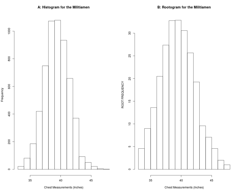
The Militiamen's Chest Dataset

Description

Militia means an army composed of ordinary citizens and not of professional soldiers. This data set is available in an 1846 book published by the Belgian statistician Adolphe Quetelet, and the data is believed to have been collected some thirty years before that.

Usage

data(chest)

Format

A data frame with 16 observations on the following 2 variables.

Chest

chest width measured in inches

Count

the corresponding frequencies

References

Velleman, P.F., and Hoaglin, D.C. (2004). ABC of Exploratory Data Analysis. Duxbury Press, Boston.

Examples

data(chest)
attach(chest)
names(chest)
militiamen <- rep(Chest,Count)
length(militiamen)
bins <- seq(33,48)
bins
bin.mids <- (bins[-1]+bins[-length(bins)])/2
par(mfrow=c(1,2))
h <- hist(militiamen, breaks = bins, xlab= "Chest Measurements (Inches)",
main= "A: Histogram for the Militiamen")
h$counts <- sqrt(h$counts)
plot(h,xlab= "Chest Measurements (Inches)",ylab= "ROOT FREQUENCY",
main= "B: Rootogram for the Militiamen")

Results

R version 3.3.1 (2016-06-21) -- "Bug in Your Hair"
Copyright (C) 2016 The R Foundation for Statistical Computing
Platform: x86_64-pc-linux-gnu (64-bit)

R is free software and comes with ABSOLUTELY NO WARRANTY.
You are welcome to redistribute it under certain conditions.
Type 'license()' or 'licence()' for distribution details.

R is a collaborative project with many contributors.
Type 'contributors()' for more information and
'citation()' on how to cite R or R packages in publications.

Type 'demo()' for some demos, 'help()' for on-line help, or
'help.start()' for an HTML browser interface to help.
Type 'q()' to quit R.

> library(ACSWR)
> png(filename="/home/ddbj/snapshot/RGM3/R_CC/result/ACSWR/chest.Rd_%03d_medium.png", width=480, height=480)
> ### Name: chest
> ### Title: The Militiamen's Chest Dataset
> ### Aliases: chest
> ### Keywords: rootogram, militiamen
> 
> ### ** Examples
> 
> data(chest)
> attach(chest)
> names(chest)
[1] "Chest" "Count"
> militiamen <- rep(Chest,Count)
> length(militiamen)
[1] 5738
> bins <- seq(33,48)
> bins
 [1] 33 34 35 36 37 38 39 40 41 42 43 44 45 46 47 48
> bin.mids <- (bins[-1]+bins[-length(bins)])/2
> par(mfrow=c(1,2))
> h <- hist(militiamen, breaks = bins, xlab= "Chest Measurements (Inches)",
+ main= "A: Histogram for the Militiamen")
> h$counts <- sqrt(h$counts)
> plot(h,xlab= "Chest Measurements (Inches)",ylab= "ROOT FREQUENCY",
+ main= "B: Rootogram for the Militiamen")
> 
> 
> 
> 
> 
> dev.off()
null device 
          1 
>